After 14 years using Microsoft On Premise BI Tools (SQL Server, Reporting Services, Integration Services and Analysis Services) Its time to embrace Business Intelligence in the cloud.
In part 1 of our initial lessons learned in Fabric blog, we looked at Data Engineering components. Our transformed dimensions and fact tables are now stored in Delta Parquet format within the Fabric Gold Lakehouse.
Now its time to look at what we can do with the Power BI Fabric functionality. Lets build our Semantic model and Reports.
The Semantic Model
Previously, the semantic model was created in Power BI Desktop. We could then create another desktop file and connect to the semantic model that had been published to the power BI Service.
With Fabric. You create the semantic model in the Fabric workspace.
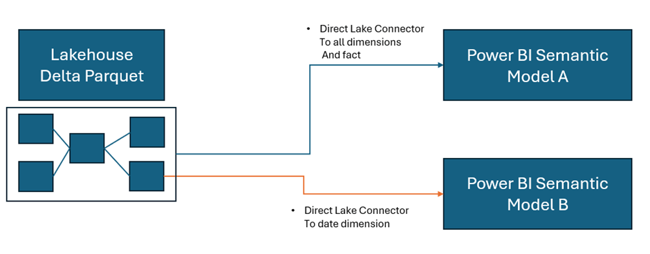
We are going to use Direct Lake connection to the Delta Parquet files. As a consequence we don’t need to create dataflows. Lets look at how this looked previously.
Without the SQL DB, with Power BI Premium. Data flows can get complex, as usually the transformations happen within the SQL database. Here they are used to simply store the data centrally before being imported into the semantic model.
You can use the data flows in multiple semantic models. For example, your date dimension could be reused in many models.
Now, we are looking at the following logic.
As a consequence, this project has been simplified to Delta Parquet and Semantic model.
In the Lakehouse, go to SQL analytics endpoint
At the bottom of the screen we have a model view. This is the Default Model view
This takes us to the Semantic Model. However, when trying to update the default model we get hit with errors
After looking at some of these issues online, it would appear that currently the ‘default’ semantic model is quite glitchy and many people are having issues with it.
People are using work arounds by creating their own semantic models rather than using the default semantic model. So currently, the default is left alone and a new semantic model is created.
Back in the Lakehouse
Choose New Semantic Model
And work in the same way as you would within your Power BI desktop file. Note that we don’t have to publish. The model auto saves.
And you can then commit your model changes to your GIT repository. Eventually creating versions of your model. You can quickly create a new report in Fabric to check your DAX as you go. This is a real change from how we used to work. Where the power BI PBIX file was simply a black box file, with no opportunities to store the code in GIT.
Notice the connections on each object
Direct Lake. Power BI directly connects to the Delta Parquet file. Just like Power BI, the file is a columnar data store, and we do not lose any DAX functionality.
Power BI Reporting
As we have seen. You can create reports directly in Fabric. A big question is, is Power BI desktop still the best thing to use?
Again I think the answer to this question is definitely yes. Although the Fabric reports can be good for quick data model testing.
Desktop allows for Offline development
Power BI Desktop can be more responsive that working on the cloud
Power BI reporting allows for better version control. You can save locally and publish to the service when ready.
Desktop integration with other external tools and services
Desktop provides more options and flexibility that reporting within Fabric.
With this in mind. Another update we can take advantage of is the Power BI PBIP (Project) desktop files. PBIP allows for version control and collaboration. Finally, Our Power BI files are broken up and code can be stored in out GIT repositories.
PBIP (the Power BI Project File)
Get Data
In Power BI Desktop you can access your Power BI semantic models
Create reports from the Semantic model(s) in Fabric.
Create the Power BI Project (PBIP)
Instead of simply saving as a pbix (black box) file, Save as a project file and see how this can really change how you work. We should see benefits like:
Items are stored in JSON format instead of being unreadable in one file
JSON text files are readable and contain the semantic model and report meta data
Source Control. Finally real source control for Power BI
Amendable by more than one person at a time
The possibility of using (CI/CD) Continuous Integration and Continuous Delivery with Power BI
Saving as a project is (Currently) in preview so lets turn it on.
Options and Settings / Options
And now we can Save as report.pbip
After saving, the project is stated in the title. Lets have a look at what has been created in Explorer
The main project file
The reporting folder
The objects within the reporting folder.
For the initial test. The pbip was save to One Drive. It needs to get added into Devops so it can be added into the full source control process along with all the Fabric code.
Azure DevOps: build pipelines for continuous integration
Ensure Fabric is already connected to Azure Devops And cloned to a local drive.
Add a powerbi folder in the local repository and all the Power BI Objects are moved here.
Using GIT Bash you can push the powerBI files up to the central repository by creating a new branch to work on
Add and commit the changes. Then Push to the cloud
Back in DevOps
We can see the Power BI Items. If you have pushed to a branch, you can then create a pull request to pull the new power BI files over into main.
To work with the file again, remember to open the (PBIP) project file from your local repository. Then you can work in Git Bash to once again. Create a new branch. Add, Commit and Push the changes.
For self service Power BI developers, this may be something that takes time to embed itself, since the process is more complex and you need to have some understanding of version control but it is really worthwhile to train your developers and build this into your standard procedures. Especially with the Silver and Gold standard (Promoted and Certified) content.
The Fabric Capacity Metrics App
Finally, lets take a quick look at the Fabric Capacity Metrics app. You need to be an admin to install and view the report.
Why is the Fabric capacity app important?
It provides insights into how the capacity is being used.
Monitoring usage patterns helps to identify how to scale resources up and down.
High usage items can be quickly identified
Installing the App
Go into your Fabric Workspace and click on the settings cog at the top right of the screen and select the governance and insights Admin Portal
I am the admin for the Fabric capacity so ensure you know who your Fabric Capacity Admin is
Click on the capacity and get the capacity ID from the URL
You can use the ID for the Capacity Metric App
In the Fabric Workspace. Go to your Power BI experience at the bottom left of the screen
Click on Apps and Get Apps
Search for the Fabric capacity App and Get it Now to install
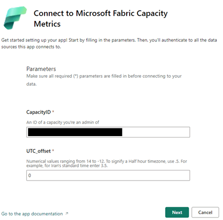
Connect to start working with the app
The screen is where you can use the capacity ID, copied from the Admin Portal. You then need to sign in and connect.
Here is where the Fabric experience falls down for me slightly currently.
The capacity app doesn’t show financial costs (Although part of the license fee. There are still costs to running spark jobs). Also, only the Fabric admin can see this information.
As a none admin user, I still want the power to be able to see my utilisation as I work with fabric.
Conclusion
The more you learn with Fabric the more exciting it gets. The next goals are to work with the Data Warehouse and the real time capabilities.
There are so many opportunities to use the Delta Lake or SQL DW as our transformation (Staging area) with Direct Lake Power BI connection. I can see Delta Lake being the option of choice to quickly to build up smaller solution projects.
As a SQL Developer, I am now a big fan of Pyspark. These two make a great tool set for the Fabric analytics engineer.
And as always with Power BI, there are exciting updates every month to look forward too. You never stop learning as an Analytics Engineer.
As at time of adding this blog. I am working towards the Fabric Engineer Certification after getting my Azure Engineer Associate some time ago. So lots more to think about. My current excitement is the real time analytics within Fabric. I.m really looking forward to trying to implement a project with this.
Any time there is a big change in technology, there is a steep learning curve to go with it. Since Microsoft announced Fabric in May 2023 We have been working hard on getting up to speed with how Fabric works and how it changes the nature of what we do.
What new architectures are available for us to work with?
How it changes working with Power BI?
How we create our staging and reporting data before loading into Power BI?
How Pipelines differ from data Factory, and pipelines in Synapse?
Keeping up with the monthly updates across Fabric
In my previous post “The Microsoft data Journey so far. From SQL Server, Azure to Fabric” I looked at my own journey working with on premises Microsoft services through to Fabric. Along with identifying all the key fabric areas.
This post is about my initial discoveries whilst actively working with Fabric, specifically using the Lake house, and ways of developing your learning within the Microsoft Fabric space.
In Part 1, we explore various topics within the Fabric Data Engineering capabilities. In Part 2, we will delve into Fabric Power BI and semantic modelling resources.
Analytics Engineer
Analytics engineer is a new title to go along with Fabric (SaaS) end to end analytics and data platform. One of the first things to do was to go through Microsoft’s Analytics Engineering learning pathway, with the aim of taking the exam.
I personally took my time with this because I wanted to get as much out of it as possible and passed the exam on the 24th of June 2024. Making me a certified Fabric Analytics Engineer.
Specialises in analytics solutions. Data engineers have a broader focus.
Collaborate closely with Data Engineers, business process knowledge owners. Analysts etc
Transforming data into reusable assets
Implementing best practices like version control and deployment
Works with lakehouses, Data Warehouses, Notebooks, Dataflows, Data pipelines, Semantic models and Reports
Skills in SQL, DAX, Pypark, ETL Tools etc
Analytics Specialist
Focuses on analysing data and data insights to support decision making
Creates reports and Dashboards and communicates findings
Identifies trends and patterns along with anomalies
Collaborates with stakeholders to understand their needs.
Skills in visualisation tools like power BI
As you can see, the Analytics Engineer is a bridge between Data Engineering and Analytics. The Analytics Specialist is sometimes seen as an end to end developer with knowledge across all of these specialties. But has a major focus on analytics solutions.
Architecture
With Fabric, we have numerous architectural options. By making strategic choices, we can eliminate the need for data copies across our architecture. Consider the standard architecture using Azure resources. A Data lake, SQL Database and Data Factory.
Here we have 2 copies of the original data. In the data Lake and the SQL Database (Because you copy the data across to transform, create your dimensions, facts etc).
And finally the same imported dims and facts created in SQL DB are imported and stored in Power BI.
This architecture works well, it allows for data scientists to use the data in the data lake and it allows for SQL Stored procedures to be put in place to process the data into the correct analytical (Star) Schemas for Power BI.
However, wouldn’t it be great if you could remove some of the data copies across the resources.
Fabric leverages the medallion architecture
Bronze layer – Our raw unprocessed data.
Silver – Cleaned and transformed data
Gold Layer – Enriched data optimised for analytics.
Even using Fabric, there are lots of opportunities to use specific resources to change your architecture dependent upon the project. For example, you could decide to use Fabrics next generation Data warehouse, designed for high performance and scalability. Excellent for big data solutions. And allows you to do cross database querying, using multiple data sources without data duplication.
However, at this point I have spent my time looking at how we can utilize the delta lake. Creating an architecture that uses Delta Parquet files. Can this be a viable solution for those projects that don’t have a need for the high level ‘big data’ performance of the Fabric Data Warehouse?
There are significant advantages here, as we are reducing the amount of duplicated data we hold.
And of course, Power BI can use Direct Lake connection, rather than Import mode. Allowing you to remove the imported model entirely from Power BI. Even better, with partitioned Delta Parquet files you can have bigger models, only using the files that you need.
This architecture has been used for some initial project work, and the Pyspark code, within Notebooks, has proved itself to be fast and reliable. As a fabric Engineer I would definitely say that if you are a SQL person its vital that you up your skills to include Pyspark.
However, with some provisos, The Data Warehouse can also utilise Direct Lake mode, so sometimes. Its literally the case of, what language do you prefer to work in. Pyspark or SQL?
Task Flows
The Fabric Task flows are a great Fabric feature, and incredibly helpful when setting up a new project.
You get to visualize your data processes
Create best practice task flows
Classify your tasks into Data Ingestion, Data Storage, Data Preparation etc
Standardise team work and are easy to navigate
Here, the Medallion flow was used, immediately giving us the architecture required to create our resources.
You can either select a previously created task to add to your task flow
Or create a new item. Fabric will recommend objects for the task
One tip from using the medallion task flow. As you can see. Bronze, Silver and Gold Data Lake houses are shown as separate activities. Currently, you can’t create one data lake and add it to each activity.
If you want to use one lake for all three areas, you need to customise the activity flow. As a result, the decision was made to have three delta lake’s working together for the project. But it may not be something you wish to do. So customising the flow may be a better option.
GIT integration
The fabric workspace comes with GIT integration, which offers a lot of benefits. With GIT, you can save your code base to your central repository, allowing for version control. Much better collaboration, better code and peer reviewing. And CI/DC automation.
There are some current issues however, especially with branching, as some branching capabilities are still in preview. For an initial test project a very basic approach was used.
Here, a new Project has been added to Devops: Debbies Training
Visual Studio
Visual Studio was used to clone the repository, but there are lots of other ways you can do this next step, For example GIT Bash.
And connect to the repository that has been created (You need to log in to see your repos)
Click clone and you will then have a local copy of the code base. It doesn’t support everything at the moment but it does support Notebooks, Reports, Semantic Models and Pipelines, which is the focus of our current learning.
Connect Devops to Fabric
Back in the Fabric Workspace go to Workspace Settings
You are now connected to Devops (Note the branch is main)
Later, we want to start using branches when the underlying Fabric logic is better, But for now, we have been using the main branch. Not ideal, but we should see this getting better a little further down the line.
You can now create your resources and be confident that your code is being stored centrally.
All you need to do is publish changes via the Fabric workspace (Source Control)
Click Commit to commit your changes and change Descriptor
Watch out for updates to this functionality. Especially branching
Pyspark and Notebooks
As a SQL developer, I have spent years writing code to create stored procedures to transform data in SQL databases.
SQL, for me is what I think of as my second language. I’m confident with it. Pyspark is fairly new to me. My biggest question was:
Using my SQL knowledge, can I think through a problem and implement that solution with Pyspark.
The answer is, yes.
As with anything. Learning new languages can be a steep learning curve. But there is lots of help out there to grips with the new language. For example, CoPilot has been incredibly useful with ideas and code. But, on the whole, you can apply what you know in SQL and use the same solutions in a Pyspark notebook.
Here are a few Tips
Pyspark, unlike SQL is CASE sensitive so you have to be much more rigorous when writing code in your notebooks.
When working with joins in Pyspark. You can significantly speed up the creation of the new data frame by using Broadcast on the smaller table. Broadcast optimizes the performance of your spark job by reducing data shuffling.
With SQL, you work with temporary tables and CTE’s (common table expressions). Dataframes replace this functionality, but you can still think of them in terms of your temporary tables.
SQL, you load the data into tables, With the Lakehouse, you load your data into files. The most common type is Parquet. It’s worth understanding the difference between Parquet and Delta Parquet. We looked at this in detail in the last blog “The Microsoft data Journey so far. From SQL Server, Azure to Fabric”. But we will look at the practicalities of both, a little later.
Unlike a SQL Stored Procedure where, during development you can leave your development work for a while. Then come back to the same state. The spark session will stop at around 20 minutes so you can’t simply leave it mid notebook. Unless you are happy to run again.
Start your session in your notebook.
Click on session status in the bottom left corner
See the session status in the bottom left corner
Here we can see the timeout period which can be reset.
Delta Parquet
When working with Parquet files. We can either save as Parquet (Saved in the files section of fabric) Or save as Delta Parquet. (Saved in the tables section of Fabric)
Always remember, if you do want to use the SQL Endpoint to run queries over your files, always save as Delta Parquet.
If you want to use the Direct Lake connector to your parquet files for Power BI Semantic Model, again, use Delta Parquet files.
One question was, if you are using a lake house and have the opportunity to create Delta Parquet. Why wouldn’t you save everything with the full Delta components of the parquet file?
There are a few reasons to still go with parquet only.
Parquet is supported across various platforms. If you share across other systems this may be the best choice.
Parquet is simple, without the ACID transaction features. This may be sufficient.
Plain parquet files can offer better performance.
Parquet files are highly efficient for storage, as they don’t have the delta parquet overheads. A good choice for archiving data.
With this in mind. Our project has followed the following logic for file creation
Dims and Facts
Always use Delta Parquet for full ACID functionality and Direct Lake connectivity to Power BI.
Audit Tables
We always keep track of our loads. When the load took place? What file was loaded? How many records? etc. Again, these are held as Delta Parquet. We can use the SQL endpoint if we want to quickly analyse the data. We can also use the Direct Lake connector for Power BI to publish the results to a report.
Even better. Our audit reports contain an issue flag. We create the logic in the Pyspark Notebook to check if there are issues. And if the flag is 1 (Yes) Power BI can immediately notify someone that there may be a problem with the data using Alerts.
Staging tables
A lot of the basic changes are held in transformed tables. We may join lots of tables together. Rename columns. Add calculated columns etc. Before loading to dims and facts. Staging tables are held as Parquet only. Basically, we only use the staging tables to load dim and fact tables. No need for the Delta overheads.
Pipelines
When you create your notebooks, Just like SQL stored Procedures, you need a way of orchestrating their runs. This is where Data Factory came in working with Azure. Now we have Pipelines in Fabric, based on the pipelines from Azure Synapse.
I have used Data factory (and its predecessor Integration Services) for many years and have worked with API’s. The copy activity. Data Mappings etc. What I haven’t used before is the Notebook activity.
There are 5 notebooks, which need to be run consecutively.
Iterate through Each Notebook
When creating pipelines, The aim is to reuse activities and objects. So, rather than having 5 activities in the pipeline. One for every notebook. We want to use 1 activity that will process all the notebooks.
In the first instance. We aren’t going to add series 5 into the Data Lake.
Create a csv file
Also get the IDs of the workspace and the notebooks. These were taken from the Fabric url’s. e.g.
The file is added into the bronze delta lake
Now we should be able to use this information in the pipeline
Create a lookup
In the pipeline we need a Lookup activity to get the information from the JSON file
Add a ForEach Activity
Drag and drop a ForEach activity onto your pipeline canvas and create an On Success Relationship between this and the Lookup.
Sequential is ticked because there are multiple rows for each notebook and we want to move through them sequentially.
Set the ‘Items’ in Settings by clicking to get to the pipeline expression builder
We are using the output.value of our lookup activity.
@activity(‘GetNotebookNames’).output.value
Configure the Notebook Activity Inside ForEach
Inside the Foreach. Add a Notebook activity
Again, click to use the Dynamic content expression builder to build
Workspace ID: @item().workspaceID
Notebook ID: @item().notebookID
Note, when you first set this up you see Workspace and Notebook Name. It changes to ID, I think this is because we are using the item() but it can be confusing.
This is the reason ID has been added into the csv file. But we still wanted the names in the file in order to better understand what is going on for error handling and testing.
@item(): This refers to the current item in the iteration which is a row. When you’re looping through a collection of items, @item() represents each individual item as the loop progresses.
.notebookID: This accesses the notebookID property of the current item. And the notebookID is a column in the csv file
Running the pipeline
You can check the inputs and outputs of each activity.
If it fails you can also click on the failure icon.
The above information can help you to create a simple pipeline that iterates through Notebooks.
There are other things to think about:
What happens if anything fails in the pipeline?
Can we audit the Pipeline Processes and collect information along the way?
Within the Notebooks, there is Pyspark code that creates auditing Delta Parquet files which contain information like: Date of Load, Number of rows, Name of activity etc. But you can also get Pipeline specific information that can also be recorded.
Currently this Pipeline can be run and it will process either 1 file or multiple files dependant upon what is added to the bronze lakehouse. The Pyspark can deal with either the very first load or subsequent loads.
With this in place, we can move forward to the Semantic Model and Power BI reporting
Conclusion
Most of the time so far has been spent learning how to use Pyspark Code to create Notebooks and our Delta Parquet files. There is so much more to do here, Data Warehousing, Delta parquet file partitioning. Real time data loading, Setting up off line development for code creation etc.
The more you learn, the more questions you have. But for the time being we are going to head off and see what we can do with our transformed data in Power BI.
In the Part 2, we will look at everything related to Power BI in Fabric.
Having lived and breathed Microsoft for over 20 years, it is important to sometimes stop and think about all the changes over those years and all the growth and learning gained from each change to the analytics space.
I started working with on premises Microsoft Products. We had a large room full of Microsoft 2000 servers and a long journey to finally upgrade to 2008 R2.
Integration Services was the orchestration tool of choice and Reporting services (SSRS) was the server based reporting tool.
We were starting to move from basic management reporting into business intelligence, especially with the introduction of SQL Server Analysis Services that became part of the environment when we finally pushed to 2008 R2.
We have come along way since those days.
On Premises Analytics
One of the biggest issues with On Premises was the upgrading to new Servers. We had a lot of servers and applications tied to those servers. Upgrading to the latest release was never easy and sometimes couldn’t be done because of the system it supported.
This led to a real disparity of servers. Some still at 2000. Some 2008 R2. A few lucky ones moving to later versions.
Another big issue specially for the analytics team was the use of the servers. Spinning up a new database needed a lot of work to make sure that whatever was required wouldn’t run out of space or memory. Because there was only a certain amount of these resources for all services.
There were examples of simply not being able to work on a project because of these restrictions.
There is nothing more frustrating as a developer to know there are later releases out there but you are stuck on an old version. Or knowing that you could do so much more with a bit more compute power or space allocation. There was no room to grow. You had to understand your full limit and work from there.
Reporting Services (SSRS)
Its interesting to look back on SSRS, Microsoft’s Paginated reporting original solution after using Power BI for so long now.
Yes it delivered fairly basic paginated reporting but it didn’t quite deliver the experience we really wanted to go with for our new Business Intelligence vision.
On Premises to Azure
A career move presented me with the opportunity to start using Azure and Power BI.
Finally, the floodgates seemed to open and new possibilities seemed to be endless. Here are just a few examples of the changes happening at this point
Azure allowing us to always be on the latest version. No more wishing that you could use SQL Server 2014 whilst stuck on 2008 R2.
Power Bi, interactive data visualisation. The complete gamechanger. We will look at that more later
Azure SQL Databases. Here we can now spin up small cheap solutions for development work. Scaling up as we go. Never needing to pay for more than we use. Even having the advantages of upping compute during peak loading times. Always being on the latest version, and so many possibilities of choice.
Serverless SQL DB for example. Great for Dev and UAT. Only unpausing compute resources when you need them.
We can still work with our SQL Skills building stored procedures to transform data.
Azure Data Lake. Secure Cloud storage for structured and unstructured data. A landing area for our data that also creates opportunities for our Data Science experts.
Azure Data Warehouse (Which upgraded to Synapse in 2019) was the offering that allows for MPP Massively parallel processing for big scale data. Along with the serverless SQL Pools (Synapse) to finally give us the chance to do analysis and transformations on the data pre the SQL Database load.
Data Factory. The Azure Data Orchestration tool. Another big gamechanger, offering so much more flexibility than Integration Services. Having a solution that can access Cloud resources and on premises resources. So much connectivity.
Power BI
Power BI is Microsoft’s modern analytics platform that gives the user the opportunity to shape their own data experience.
To drill through to new detail.
Drill down into hierarchies.
Filter data.
Use AI visuals to gain more insight.
Better visuals
And at the heart of everything. The Power BI Tabular storage model. The Vertipaq engine, Creating reporting that can span over multiple users all interacting with these report pages. Each user sending queries to the engine at speed.
I have worked with Analysis Services in the past, along with SSRS. Creating Star Schemas sat in columnar storage without needing to set up Analysis Services was a huge win for me as it was a much easier process.
Of course, you can’t talk about Power BI without understanding how different each license experience is. From the Power BI Pro Self Service environment, through to Power BI Premium Enterprise Level License.
There has been a lot of changes and Premium continues to create fantastic additional functionality. Premium sits on top of the Gen 2 Capacity offering larger model sizes. More compute. Etc.
As a take away. When working with Pro, you should always work with additional Azure resources, like Azure SQL DB, Integration Services etc to get the best end product.
With Azure and Power BI we have worked with the recommended architectures and produced quality analytics services time and time again. But, there were still some issues and pain points along the way.
And this is where Fabric comes in.
Fabric
Fabric is the (SaaS) Software as a Service Solution, pulling together all the resources needed for analytics, data science and real time reporting. Fabric concentrates on these key areas to provide an all in one solution.
On the whole, for an analytics project, working with customers, our (basic) architecture for analytics projects was as follows:
Extract data into a Data Lake using Integration Services on a Schedule
Load the data into SQL Server Database
Transform the data into STAR schema (Facts and Dimensions) for Power BI analytics
Load the data into Power BI (Import mode where ever possible. But obviously there are opportunities for Direct Query, and Composite modelling for larger data sets)
We can see here that the data is held in multiple areas.
Synapse starts to address this with the Serverless SQL Pools. We can now create Notebooks of code to transform our data on the file itself. Rather than in the SQL Database on the fully structured data.
Fabric has completely changed the game. Lets look into how in a little more detail.
Medallion architecture
First of all, we need to understand the architectures we are working with. The medallion architecture gives us specific layers
Gold – Our landing area. The data is added to the lake. As is. No Processing
Silver – The Data is transformed and Processed
Gold – the data is structured in a way that can be used for Analytics. The Star schema for Power BI.
Fabric allows us to work with the medallion architecture seamlessly. And as announced at Microsoft build in May of this year. We now have Task Flows to organise and relate resources. The Medallion architecture is one of the Flows that you can immediately spin up to use.
Delta Lake
The Delta lake enhances Data Lake performance by providing ACID transactional processes.
A – Atomicity, transactions either succeed or fail completely.
C – Consistency, Ensuring that data remains valid during reads and writes
I – Isolation, running transactions don’t interfere with each other
D – Durability, committed changes are permanent. Uses cloud storage for files and transaction logs
Delta Lake is the perfect storage for our Parquet files.
Notebooks
Used to develop Apache Spark jobs so we can now utilise code such as Pyspark and transform the data before adding into a new file ready to load.
Delta Parquet
Here is where it gets really interesting. In the past our data has been held as CSV’s, txt etc. Now we can add in Parquet files into our architecture.
Parquet is an open source, columnar storage file format.
The Power BI data model is also a columnar data store. This creates really exciting opportunities to work with larger models and have the full suite of Power BI DAX and functionality available to us.
But Fabric also allows us to create our Parquet Files as Delta Parquet, adhering to the ACID guarantees.
The Delta is and additional layer over Parquet that allows us to do such things as time travel with the transaction log. We can hold versions of the data and run VACUUM to remove old historical files not required anymore.
Direct Lake Mode
Along with Parquet we get a new Power BI Import mode to work with. Direct Lake allows us to connect directly to Delta Parquet Files and use this columnar data store instead of the Power BI Import mode columnar model.
This gives us a few advantages:
Removes an extra layer of data
Our data can be partitioned into multiple files. And Power BI can use certain partitions. Meaning we can have a much bigger model.
Direct Query, running on top of a SQL DB is only as quick as the SQL DB. And you can’t use some of the best Power BI Capabilities like DAX Time Intelligence. With Direct Lake you get all the functionality of an Import model.
SQL Analytics Endpoints
If you are a SQL obsessive, like myself you can analyse the data using the SQL analytics endpoint within a file. No need to process into a structured SQL Database
Data Warehouse
Another one for SQL obsessives and for Big Data reporting needs. There will be times when you still want to serve via a structured Data Warehouse.
Conclusion
Obviously this is just a very brief introduction to Fabric and there is so much more to understand and work with. However using the Medallion architecture we can see a really substantial change in the amount of data layers we have to work with.
And the less we have of data copies, the better our architecture will be. There are still a lot of uses for the Data Warehouse but for many smaller projects, this offers us so much more.
Its been a long journey and knowing Microsoft, there will be plenty more fantastic new updates coming. Along the way, I would say that these three ‘jumps’ were the biggest game changes for me, and I can’t wait to see what Fabric can offer.
Now we have updated our ProcessedFiles delta parquet, we can update the dimensions accordingly.
It might be nice to have another delta parquet file here we can use to collect meta data for dims and facts.
We will also want the processedDate in each dim and fact table.
We are going to start with Delta Load 2. So. Series 1 and 2 have already been loaded. We are now loading Series 3 (This shows off some of the logic better)
Dim Contestant.
Bring back the list of Processed Files from ProcessedFiles
Immediately we have a change to the code because its delta Parquet and not Parquet
# Define the ABFS path to the Delta table
delta_table_path = "abfss://########-####-####-####-############@onelake.dfs.fabric.microsoft.com/########-####-####-####-############/Tables/processedfiles"

# Read the Delta table
dflog = spark.read.format("delta").load(delta_table_path)

# Filter the DataFrame
df_currentProcess = dflog[dflog["fullyProcessedFlag"] == 0][["Filename"]]

# Display the DataFrame
display(df_currentProcess)
New Code Block Check processed Files
In the previous code, we:
Create a new taskmaster schema to load data into
Loop through the files and add data to the above schema
Add the current process data into CurrentProcessedTMData.parquet.
Add the ProcessDate of the Taskmaster transformed data
We know at some point that we are having issues with the fact table getting duplicate series so we need to check throughout the process where this could be happening.
Change the processDate from being the TaskmasterTransformed process date, in case this was done on an earlier day. We want the current date here to ensure everything groups together.
We could also set up this data so we can store it in our new Delta parquet Log
Because we are also adding process date to the group. we need to be careful. minutes and seconds could create extra rows and we don’t want that
We also know that we are doing checks on the data as it goes in. And rechecking the numbers of historical data. so we need a flag for this
from pyspark.sql import functions as F

workspace_id = "########-####-####-####-############"
lakehouse_id = "########-####-####-####-############"

# Define the file path
file_path = f"abfss://{workspace_id}@onelake.dfs.fabric.microsoft.com/{lakehouse_id}/Files/Data/Silver/Log/CurrentProcessedTMData.parquet"

# Read the Parquet file
dfCheckCurrentProc = spark.read.parquet(file_path)

# Add the new column
dfCheckCurrentProc = dfCheckCurrentProc.withColumn("sequence", F.lit(1))
dfCheckCurrentProc = dfCheckCurrentProc.withColumn("parquetType", F.lit("parquet"))
dfCheckCurrentProc = dfCheckCurrentProc.withColumn("analyticsType", F.lit("Transformation"))
dfCheckCurrentProc = dfCheckCurrentProc.withColumn("name", F.lit("CurrentProcessedTMData"))
# Set the date as the current date
dfCheckCurrentProc = dfCheckCurrentProc.withColumn("processedDate", current_date())
dfCheckCurrentProc = dfCheckCurrentProc.withColumn("historicalCheckFlag", F.lit(0))
dfCheckCurrentProc = dfCheckCurrentProc.withColumn("raiseerrorFlag", F.lit(0))

# Select the required columns and count the rows
dfCheckCurrentProc = dfCheckCurrentProc.groupBy("sequence","parquetType","analyticsType","name","source_filename", "processedDate","historicalCheckFlag","raiseerrorFlag").count()

# Rename the count column to TotalRows
dfCheckCurrentProc = dfCheckCurrentProc.withColumnRenamed("count", "totalRows")

# Show the data
display(dfCheckCurrentProc)
current_date() gets the current date. We only have date in the grouped auditing table. date and time can go into the dimension itsself in the process date.
sequence allows us to see the sequence of dim and fact creation
parquetType is either Parquet or Delta Parquet for this project
analyticsType is the type of table we are dealing with
historicalCheckFlag. Set to 0 if we are looking at the data being loaded. 1 if the checks are against older data.
raiseErrorflag if there looks like we have any issues. This can be set to 1 and someone can be alerted using power BI Reporting.
It would be really good to also have a run number here because each run will consist of a number of parquet files. In this case parquet and delta parquet
Get ContestantTransformed data
A small update here. Just in case, we use distinct to make sure we only have distinct contestants in this list
# Ensure the DataFrame contains only distinct values
dfc = dfc.distinct()
Merge Contestants and Taskmaster data
This is the point where we create the Contestant Dimension. the processDate to the current date and alias to to just processedTime.
from pyspark.sql.functions import col, current_date
from pyspark.sql import SparkSession, functions as F

df_small = F.broadcast(dfc)


# Perform the left join
merged_df = dftm.join(df_small, dftm["Contestant"] == df_small["Name"], "left_outer")\
                .select(
                    dfc["Contestant ID"],
                    dftm["Contestant"].alias("Contestant Name"),
                    dftm["Team"],
                    dfc["Image"],
                    dfc["From"],
                    dfc["Area"],
                    dfc["country"].alias("Country"),
                    dfc["seat"].alias("Seat"),
                    dfc["gender"].alias("Gender"),
                    dfc["hand"].alias("Hand"),
                    dfc["age"].alias("Age"),
                    dfc["ageRange"].alias("Age Range"),
                    current_timestamp().alias("processedTime"),
                ).distinct()


# Show the resulting DataFrame
merged_df.show()
Add the Default row
This changes because we have a new column that we need to add.
from pyspark.sql import SparkSession,Row
from pyspark.conf import SparkConf
from pyspark.sql.functions import current_timestamp


workspace_id = "########-####-####-####-############"
lakehouse_id = "########-####-####-####-############"

path_to_parquet_file = (f"abfss://{workspace_id}@onelake.dfs.fabric.microsoft.com/{lakehouse_id}/Tables/dimcontestant")

# Check if the Delta Parquet file exists
delta_file_exists = spark._jvm.org.apache.hadoop.fs.FileSystem.get(spark._jsc.hadoopConfiguration()).exists(spark._jvm.org.apache.hadoop.fs.Path(path_to_parquet_file))

if delta_file_exists:
    print("Delta Parquet file exists. We don't need to add the NA row")
else:

    # Add a Default row
    # Create a sample DataFrame
    data = [(-1, "Not Known","Not Known","Not Known","Not Known","Not Known","Not Known","0","NA","0","0","0")]
    columns = ["Contestant ID", "Contestant Name", "Team","Image","From","Area","Country","Seat","Gender","Hand","Age","Age Range"]
    new_row  = spark.createDataFrame(data, columns)

    # Add the current timestamp to the ProcessedTime column
    new_row = new_row.withColumn("ProcessedTime", current_timestamp())

    # Union the new row with the existing DataFrame
    dfContfinal = dfContfinal.union(new_row)

    # Show the updated DataFrame
    dfContfinal.show(1000)

    print("Delta Parquet file does not exist. Add NA Row")
The above screen show is for Series 1 and 2. Just to show you that the row is created if its the first time.
All the process dates are the same (at least the same day) ensuring everything will be grouped when we add it to the audit delta parquet table.
However, this is displayed for our 2nd load for series 3 (2nd load)
Check the new data that has been loaded into the delta parquet.
Checking the data, checks the dimension that has been created as delta parquet This is the last code section and we want to build more in after this
Get the Contestant Names and Source Files of the Current Load
Because we can process either 1 file alone, or multiple files. we need to get the source file name AND the contestant name at this point.
#Get just the contestant name and source File name from our currrent load
df_contestant_name = dftm.selectExpr(“`Contestant` as contestantNameFinal”, “`source_filename` as sourceFileNameFinal”).distinct()
df_contestant_name.show()
For the audit we need to know what our current Contestants are and who are the Contestants we have previously worked with. Also the original file they below too.
We took this information from an earlier dataframe when we loaded the source file to be used to create the dimension. This still contains the source file name. The Dimension does not contain the file name any more.
Join df_contestant_name to dfnewdimc to see what data is new and what data has been previously loaded
from pyspark.sql.functions import broadcast, when, col

df_joined = dfnewdimc.join(
    df_contestant_name,
    dfnewdimc.ContestantName == df_contestant_name.contestantNameFinal,
    how='left'
)
# Add the currentFlag column
df_joined2 = df_joined.withColumn(
    "historicalCheckFlag",
    when((col("contestantNameFinal").isNull()) & (col("ContestantKey") != -1), 1).otherwise(0))

# Drop the ContestantNameFinal column
df_joined3 = df_joined2.drop("contestantNameFinal")

#If its an audit row set sourceFileNameFinal to Calculated Row
df_joined4 = df_joined3.withColumn(
    "sourceFileNameFinal",
    when((col("sourceFileNameFinal").isNull()) & (col("ContestantKey") == -1), "Calculated Row")
    .otherwise(col("sourceFileNameFinal"))
)

# Show the result
display(df_joined4)
This joins the name we have just created to the data we are working with so we can set the historicalCheckFlag. For the first load everything is 0 because they are current.
In this load we can see some 1’s These are records already in the system and don’t match to our current load.
This file also now contains the source_filename
If its a default row, there will be no source filename so we set to calculated Row instead
Creating Dim Audit row
from pyspark.sql import functions as F
from pyspark.sql import SparkSession
from pyspark.sql.types import StructType, StructField, StringType, IntegerType, TimestampType
from pyspark.sql import DataFrame

# Add the new column

dfdimaudit = df_joined4.withColumn("sequence", F.lit(2))

dfdimaudit = dfdimaudit.withColumn("parquetType", F.lit("Delta parquet"))

dfdimaudit = dfdimaudit.withColumn("analyticsType", F.lit("Dimension"))

dfdimaudit = dfdimaudit.withColumn("name", F.lit("Dim Contestant"))

# Extract the date from source_processedTime
dfdimaudit  = dfdimaudit.withColumn("processedDate", F.to_date("processedTime"))
dfdimaudit =  dfdimaudit.withColumn("raiseerrorFlag", F.lit(0))

# Select the required columns and count the rows
dfdimauditgr = dfdimaudit.groupBy("sequence","parquetType","analyticsType","name", "sourceFileNameFinal","processedDate","historicalCheckFlag","raiseerrorFlag").count()


# Alias sourceFileNameFinal to sourceFileName
dfdimauditgr = dfdimauditgr.withColumnRenamed("sourceFileNameFinal", "source_filename")

# Alias count to totalRowsdfdimauditgr = dfdimauditgr.withColumnRenamed("count", "totalRows")

# Show the data
display(dfdimauditgr)
The files are grouped on processed time. So we need to deal with this accordingly so set date and time to just date using to_date() (To avoid minutes and seconds causing issues)
Our default row is set against, calculated Row.
The null source file name is the total count of our historical records
We are going to append the dim audit to the initial current processed audit so they both need exactly the same columns and these are
sequence
parquetType
analyticsType
name
source_filename
processedDate
totalRows
historicalCheckFlag
raiseerrorFlag
and we have the correct source file name. Even if we process multiple files.
Add Historical Data Check to null source filename
Append the audit for the transformation data and Dimension data
# Append the current processed transformation file(s) audit row with the dimension audit

audit3_df = dfCheckCurrentProc.unionByName(dfdimauditgr)

display(audit3_df)
With the S3 file loaded we can see
Transformation rows for series 3.
Dimension rows for Contestant S3
The historical row count of all series already in the dimension.
Create Batch numbers for the audit.
If its the first time we run this process. Set to 0. Else set to the Match Last Batch No + 1
from pyspark.sql.functions import lit

# Function to check if a table exists
def table_exists(spark, table_name):
    return spark._jsparkSession.catalog().tableExists(table_name)

# Table name
table_name = "SilverDebbiesTraininglh.processeddimfact"

if table_exists(spark, table_name):

    # If the table exists, get the max batchno
    df = spark.table(table_name)
    max_batchno = df.agg({"batchno": "max"}).collect()[0][0]
    next_batchno = max_batchno+1

    # Add the batchNo column with a value of 0
    audit3_df = audit3_df.withColumn("batchNo", lit(next_batchno))

    print(f"processedDimFact data already exists. Next batchno: {next_batchno}")
    display(audit3_df)
else:

    # Add the batchNo column with a value of 0
    audit3_df = audit3_df.withColumn("batchNo", lit(0))


    # Reorder columns to make batchNo the first column
    columns = ['batchNo'] + [col for col in audit3_df.columns if col != 'batchNo']
    audit3_df = audit3_df.select(columns)

    print("Table does not exist. Add Batch No 0")

    display(audit3_df)
The following gives more information about the code used.
def table_exists(spark, table_name): defines a function named table_exsts that takes two parameters. the spark session object and the table name
Next we define a function named table_exists that will look for the table name
spark._jsparkSession.catalog() accesses the spark session catalogue which contains metadata about the entities in the spark session.
Basically, this is checking if the table name exists in the spark session catalogue. It it does we get the match Batch no from the table. Add 1 and add that as the column next_batchno
If its false we start batchno at 0
How does the column reordering work?
[‘batchNo’]: This creates a list with a single element, ‘batchNo’. This will be the first column in the new order.
[col for col in audit3_df.columns if col != ‘batchNo’]: This is a list comprehension that iterates over all the columns in audit3_df and includes each column name in the new list, if removes ‘batchNo’ from the list.
List Comprehension: Create lists by processing existing lists (Like columns here) into a single line of code.
Combining the lists: The + operator concatenates the two lists. So, [‘batchNo’] is combined with the list of all other columns, resulting in a new list where ‘batchNo’ is the first element, followed by all the other columns in their original order.
And here we can see in Load 2 we hit the if section of the above code. Our batch no is 1 (Because the first load was 0)
Reset totalRows to Integer
Found that totalRows was set to long again so before adding into delta parquet. reset to int.
Bring back the processeddimFact before saving with the new rows
Before saving the new audit rows we want to know if there are any issues. This means we need the data. However we also need to deal with the fact that this may be the first process time and there won’t be a file to check.
table_path = "abfss://########-####-####-####-############@onelake.dfs.fabric.microsoft.com/########-####-####-####-############/Tables/processeddimfact"
table_exists = DeltaTable.isDeltaTable(spark, table_path)

if table_exists:
    # Load the Delta table as a DataFrame
    dfprocesseddimfact = spark.read.format("delta").table("SilverDebbiesTraininglh.processeddimfact")

    # Display the table
    dfprocesseddimfact.show()  # Use show() instead of display() in standard PySpark

    # Print the schema
    dfprocesseddimfact.printSchema()

    print("The Delta table SilverDebbiesTraininglh.processeddimfact exists. Bring back data")
else:

    # Define the schema
    schema = StructType([
        StructField("batchNo", IntegerType(), nullable=False),
        StructField("sequence", IntegerType(), nullable=False),
        StructField("parquetType", StringType(), nullable=False),
        StructField("analyticsType", StringType(), nullable=False),
        StructField("name", StringType(), nullable=False),
        StructField("source_filename", StringType(), nullable=True),
        StructField("processedDate", DateType(), nullable=True),
        StructField("historicalCheckFlag", IntegerType(), nullable=False),
        StructField("raiseerrorFlag", IntegerType(), nullable=False),
        StructField("totalRows", IntegerType(), nullable=False)
    ])

    # Create an empty DataFrame with the schema
    dfprocesseddimfact = spark.createDataFrame([], schema)

    dfprocesseddimfact.show()

    print("The Delta table SilverDebbiesTraininglh.processeddimfact does not exist. Create empty dataframe")
If there is no data we can create an empty schema.
Get the Total of Dim Contestant rows (None Historical)
from pyspark.sql.functions import col, sum

# Filter the dataframe where name is "Dim Contestant"
filtered_df = dfprocesseddimfact.filter((col("Name") == "Dim Contestant") & (col("historicalCheckFlag") == 0)& (col("source_filename") != "Calculated Row"))

display(filtered_df)


# Calculate the sum of TotalRows
total_rows_sum = filtered_df.groupBy("Name").agg(sum("TotalRows").alias("TotalRowsSum"))

# Rename the "Name" column to "SelectedName"
total_rows_sum = total_rows_sum.withColumnRenamed("Name", "SelectedName")


display(total_rows_sum)

# Print the result
print(f"The sum of TotalRows where name is 'Dim Contestant' is: {total_rows_sum}")
Both Initial (None Historical Loads) equal 10
Get Historical Rows from our latest process and join to total Loads of the previous Load
#Join total_rows_sum to audit3_df
from pyspark.sql.functions import broadcast

# Broadcast the total_rows_sum dataframe
broadcast_total_rows_sum = broadcast(total_rows_sum)

# Perform the left join
df_checkolddata = audit3_df.filter(
    (audit3_df["historicalCheckFlag"] == 1) & (audit3_df["source_filename"] != "Calculated Row")
    ).join(
    broadcast_total_rows_sum,
    audit3_df["name"] == broadcast_total_rows_sum["SelectedName"],
    "left"
)

# Show the result
display(df_checkolddata)
So Series 1 and 2 have 10 contestants. After S3 load there are still 10 contestants. Everything is fine here. The historical records row allows us to ensure we haven’t caused any issues.
Set Raise Error Flag if there are issues
And now we can set the error flag if there is a problem which can raise an alert.
from pyspark.sql.functions import col

# Assuming df is your DataFrame
total_rows_sum = df_checkolddata.agg({"TotalRowsSum": "sum"}).collect()[0][0]
total_rows = df_checkolddata.agg({"totalRows": "sum"}).collect()[0][0]

# Check if TotalRowsSum equals totalRows
if total_rows_sum == total_rows:
    print("No issue with data")

else:
    df_checkolddata = df_checkolddata.withColumn("raiseerrorFlag", lit(1))

    print("Old and historical check does not match. Issue. Set raiseerrorFlag = 1")

# Show the updated DataFrame
df_checkolddata.show()
raiseerrorFlag is still 0
Remove the historical check row if there is no error
from pyspark.sql.functions import col

# Alias the DataFrames
audit3_df_alias = audit3_df.alias("a")
df_checkolddata_alias = df_checkolddata.alias("b")

# Perform left join on the name column and historicalCheckFlag
df_audit4 = audit3_df_alias.join(df_checkolddata_alias,
                              (col("a.name") == col("b.name")) &
                              (col("a.historicalCheckFlag") == col("b.historicalCheckFlag")),
                              how="left")

# Select only the columns from audit3_df and TotalRowsSum from df_checkolddata, and alias historicalCheckFlag
df_audit5 = df_audit4.select(
    "a.*",
    col("b.raiseerrorFlag").alias("newraiseErrorFlag")
)


# Filter out rows where newraiseerrorflag is 0 because its fine. We don';'t need to therefore know about the historical update
df_audit6  = df_audit5.filter((col("newraiseErrorFlag") != 0) | (col("newraiseErrorFlag").isNull()))

# Remove the columns newraiseerrorflag
df_audit7 = df_audit6.drop("newraiseErrorflag")


# Show the result
display(df_audit7)
the historical row has been removed. if there isn’t a problem, there is no need to hold this record.
If the data has multiple audit rows. Flag as an issue. Else remove
# Count the number of rows where ContestantName is "Not Known"
dfcount_not_known = dfnewdimc.filter(col("ContestantName") == "Not Known").count()

# Print the result
print(f"Number of rows where ContestantName is 'Not Known': {dfcount_not_known}")

# Check if count_not_known is 1
if dfcount_not_known == 1:
    # Remove row from df_audit7 where source_filename is "CalculatedRow"
    df_audit8 = df_audit7.filter(col("source_filename") != "Calculated Row")

    print(f"1 dim audit row. We can remove the row from the audit table")

else:
    # Set source_filename to "Multiple Calculated Rows issue"
    df_audit8 = df_audit7.withColumn("source_filename",
                                     when(col("source_filename") == "Calculated Row",
                                          lit("Multiple Calculated Rows issue"))
                                     .otherwise(col("source_filename")))


    print(f"multiple dim audit row. We can specify this in the audit table")

# Show the updated df_audit7
df_audit8.show()
The Audit rows has now been removed. Unless there is an issue we don’t need it. this will be useful if we accidentally process multiple audit rows into the table.
Save as Delta Parquet
from delta.tables import DeltaTable

#You can also add the none default daya lake by clicking +Lakehouse
audit3_df.write.mode("append").option("overwriteSchema", "true").format("delta").saveAsTable("SilverDebbiesTraininglh.processedDimFact")

# Print a success message
print("Parquet file appended successfully.")
And save the data as a Delta Parquet processedDimFact in our Silver transform layer.
We can use both of these Delta Parquet Files later.
Check processdimfact
Dim Contestant is complete for now. But we will come back later to update the code.
Dim Episode
Create Episode Dim
Small change. We are adding processedTime as the current date and time.
from pyspark.sql.functions import current_timestamp

dftmEp = dftm.select("Series","Episode No" ,"Episode Name").distinct()

# Add the current timestamp as processedTime
dftmEp = dftmEp.withColumn("processedTime", current_timestamp())

dftmEp = dftmEp.orderBy("Series", "Episode No")

display(dftmEp)
Add a Default row
Just like Contestant. We need ProcessedTime adding
from pyspark.sql.functions import current_timestamp
 # Add the current timestamp to the ProcessedTime column
    new_row = new_row.withColumn("ProcessedTime", current_timestamp())
Again, Here is the screenshot taken on the first load of S1 and S2
And our S3 Load 2 hits the if block and no default row is created
Get the Series, Episode Name and Source File of the Processed data
#Get just the series, Episode Name and source_filename from our current load

df_SeEp = dftm.selectExpr("`Series` as SeriesFinal", "`Episode Name` as EpisodeFinal", "source_filename").distinct()

display(df_SeEp)
` are used in PySpark to handle column names that contain special characters, spaces, or reserved keywords.
Join df_SeEp to dfnewdimt
Join the list pf currently processed series and episodes to everything in the dimension so far (the data frame we created when we checked the dim
from pyspark.sql.functions import broadcast, when, col

# Broadcast df_contestant_name and perform the left join
df_joined = dfnewdimt.join(
    broadcast(df_SeEp),
    (dfnewdimt.Series == df_SeEp.SeriesFinal) & (dfnewdimt.EpisodeName == df_SeEp.EpisodeFinal),
    "left"
)
# Add the currentFlag column
df_joined2 = df_joined.withColumn("historicalCheckFlag", when(col("SeriesFinal").isNull(), 1).otherwise(0))

# Drop the ContestantNameFinal column
df_joined3 = df_joined2.drop("SeriesFinal").drop("EpisodeFinal")

#If its an audit row set sourceFileNameFinal to Calculated Row
df_joined4 = df_joined3.withColumn(
    "source_filename",
    when((col("source_filename").isNull()) & (col("EpisodeKey") == -1), "Calculated Row")
    .otherwise(col("source_filename"))
)

# Show the result
display(df_joined4)
All historicalCheckFlags are set to 0 if its the current Load (s3). 1 when there is no match and its historical data. the source_filename from df.SeEp has been left in the result which can be used later.
Again we have set the Episode Keys source_filename to “calculated Row” because there is no source to join this one record on by the series and episode name.
Add audit row
At the end of the process. We will add an audit row
from pyspark.sql import functions as F

# Add the new column
dfdimaudit = df_joined4.withColumn("sequence", F.lit(3))

dfdimaudit = dfdimaudit.withColumn("parquetType", F.lit("Delta parquet"))

dfdimaudit = dfdimaudit.withColumn("analyticsType", F.lit("Dimension"))

dfdimaudit = dfdimaudit.withColumn("name", F.lit("Dim Episode"))

# Extract the date from source_processedTime
dfdimaudit  = dfdimaudit.withColumn("processedDate", F.to_date("processedTime"))

dfdimaudit =  dfdimaudit.withColumn("raiseerrorFlag", F.lit(0))

# Select the required columns and count the rows
dfdimauditgr = dfdimaudit.groupBy("sequence","parquetType","analyticsType","name", "source_filename","processedDate","historicalCheckFlag","raiseerrorFlag").count()

# Alias count to totalRows
dfdimauditgr = dfdimauditgr.withColumnRenamed("count", "totalRows")

# Show the data
display(dfdimauditgr)
for Load 2 we have 5 records in the current load with the source filename set. The historical load of 11 and the calculated Audit -1 row.
Bring back our processeddimfact data
from delta.tables import DeltaTable
from pyspark.sql.functions import col, max

# Load the Delta table as a DataFrame
dfprocesseddimfact = spark.read.format("delta").table("SilverDebbiesTraininglh.processeddimfact")

# Find the maximum BatchNo
max_batch_no = dfprocesseddimfact.agg(max("BatchNo")).collect()[0][0]

# Filter the DataFrame to include only rows with the maximum BatchNo
dfprocesseddimfact = dfprocesseddimfact.filter(col("BatchNo") == max_batch_no)

# Display the table
display(dfprocesseddimfact)
dfprocesseddimfact.printSchema()
Here we find the max batch number and then filter our data frame to only give us the max batch number which is the one we are working on. (Because at this point, we are in the middle of a batch of dims and facts)
We just want that distinct Max Batch number for the next process
Join to our Dim Episode Audit row to bring in the batch number via Left outer join
# Alias the dataframes
dfdimauditgr_alias = dfdimauditgr.alias("dfdimauditgr")
distinct_batch_no_alias = distinct_batch_no.alias("dfprocesseddimfact")

# Perform inner join
audit2_df = dfdimauditgr_alias.crossJoin(distinct_batch_no_alias)

# Select specific columns
audit2_df = audit2_df.select(
    distinct_batch_no_alias.batchNo,
    dfdimauditgr_alias.sequence,
    dfdimauditgr_alias.parquetType,
    dfdimauditgr_alias.analyticsType,
    dfdimauditgr_alias.name,
    dfdimauditgr_alias.source_filename,
    dfdimauditgr_alias.totalRows,
    dfdimauditgr_alias.processedDate,
    dfdimauditgr_alias.historicalCheckFlag,
    dfdimauditgr_alias.raiseerrorFlag
)

audit2_df = audit2_df.distinct()

# Show result
display(audit2_df)
The cross join (Cartesian Join) is because there is only 1 batch number set in distinct_batch_no (the Max Batch number is the one we are working on) So no need to add join criteria.
Set totalRows to Int
Once again TotalRows needs setting to Int
Get the processeddimfact data
# Load the Delta table as a DataFrame
    dfprocesseddimfact = spark.read.format("delta").table("SilverDebbiesTraininglh.processeddimfact")

    # Display the table
    dfprocesseddimfact.show()  # Use show() instead of display() in standard PySpark

    # Print the schema
    dfprocesseddimfact.printSchema()
    # Load the Delta table as a DataFrame
    dfprocesseddimfact = spark.read.format("delta").table("SilverDebbiesTraininglh.processeddimfact")

    # Display the table
    dfprocesseddimfact.show()  # Use show() instead of display() in standard PySpark

    # Print the schema
    dfprocesseddimfact.printSchema()
We will need this to check our historical checked data against the original update
Get the total rows of our None historical rowsthat have been previously loaded
Same logic as Contestant
Join Historical records with new audit to see if the numbers have changed
No changes to the old numbers.
Set raiseerrorFlag if there are issues
There are no issues
If no issues. Record is removed
As there are no issues the record is removed
If Audit row -1 is only in once. No need to hold the audit row
Append into processeddimfact
And check the data looks good
We head off into Dim Task now and here is where we hit some issues. We need to add more code into the process.
Dim Task
checking the count of rows between the original load, and the historical check
When we count the rows of processed data they come to 64. But when we run the check again it comes to 65. Which would trigger the raise error flag. And this is why
dfnewdimt_filtered = dfnewdimt.filter(dfnewdimt["Task"] == "Buy a gift for the Taskmaster")
display(dfnewdimt_filtered)
I settled on Task and TaskOrder to create the unique row. However this isn’t the case. we have two series where our Task and Task Order are identical.
What we really want is one record in the dimension applied to the correct seasons in the fact table. Not a duplicate like we have above.
The following code is adding Series 3 to both “Buy a gift for the taskmaster” and is consequently undercounting.
Series three is a good opportunity to update the logic as we know there is a record already added from season 2
Bring back old dimTask
from delta.tables import DeltaTable
from pyspark.sql import SparkSession
from pyspark.sql.types import StructType, StructField, StringType, IntegerType, TimestampType

# Initialize Spark session
#spark = SparkSession.builder.appName("DeltaTableCheck").getOrCreate()

# Path to the Delta table
table_path = "abfss://########-####-####-####-############@onelake.dfs.fabric.microsoft.com/########-####-####-####-############/Tables/dimtask"

# Check if the Delta table exists
if DeltaTable.isDeltaTable(spark, table_path):
    # Load the Delta table as a DataFrame
    dfprevdimt = spark.read.format("delta").load(table_path)

else:
    # Define the schema for the empty DataFrame
    schema = StructType([
        StructField("Task", StringType(), True),
        StructField("TaskOrder", IntegerType(), True),
        StructField("TaskType", StringType(), True),
        StructField("Assignment", StringType(), True),
        StructField("ProcessedTime", TimestampType(), True)
    ])

    # Create an empty DataFrame with the specified schema
    dfprevdimt = spark.createDataFrame([], schema)

    print("no dim. Create empty dataframe")

# Display the DataFrame
dfprevdimt.show()
If its the first time, create an empty dataset. else bring back the dataset
Join new Tasks to all the Previously added tasks
The decision has been made to use all the columns in the join, Just in case a Task has a different assignment or Type.
Our Task that we know is identical for Series 2 and 3 appears. We use the dftm dataframe. This contains the data before we create the distinct dimension, as this contains source_filename. Inner Join only brings back the matching records.
Add this to a Delta Parquet File
We can now have a static item we can use later. and we can report on these items
If task already exists. Remove from the new load
from pyspark.sql.functions import col,current_timestamp

# Alias the DataFrames
dfprevdimt_df_alias = dfprevdimt.alias("old")
dftm_alias = dftm.alias("new")

# Perform left join on the name column and historicalCheckFlag
dftmdupRemoved = dftm_alias.join(dfprevdimt_df_alias,
                              (col("new.Task") == col("old.Task")) &
                              (col("new.Task Order") == col("old.TaskOrder"))&
                              (col("new.Task Type") == col("old.TaskType"))&
                              (col("new.Assignment") == col("old.Assignment")),
                              how="Left_anti")


#And reset the dimension
dfTasksdupRemoved = dftmdupRemoved.select("Task","Task Order" ,"Task Type", "Assignment").distinct()

# Add the current timestamp as processedTime
dfTasksdupRemoved = dfTasksdupRemoved.withColumn("processedTime", current_timestamp())

# Show the result
display(dfTasksdupRemoved)
The left anti join bring back records that exist in the new data frame and removes anything that also exists in the pre existing data
dtfm is again used so we have to reset the dimension.
dfTasksdupRemoved now becomes our main dataframe so we need to ensure its used across the Notebook where neccessary
We then go on to create the default row (If its never been run before) and keys
Add a Default Row
Code changed to use dfTasksdupRemoved
Create the Task Key
Again, we have had a change to code to use the updated dataframe
Get Task details from current load
Previously, This was just Task and Order but we know that we need more in the join.
Create a historical Record check
Buy a gift for the Taskmaster is flagged as historical (Its in Series 2) and we have removed it from series 3. And we have added this information to a Delta Parquet.
We have also added more join criteria.
Create the Audit Rows
Add a value into source filename if full because its a historical record
Bring back the ProcessedDimfact
Get the Current batch
Join the batch number into the dataframe
Load the processed Dim Fact
Count the rows
Total Rows is correct at 65
Add the Rows of the historical check against rows that were originally processed
These now match
If Issue. Set RaiseErrorFlag = 1
No issues
Remove historical check if there are no issues
Check that there aren’t multiple rows in the data for the default -1 row. If all ok. remove default row from audit
And append the data into processeddimfact.
There is other logic to consider here. Imagine if we loaded in Series 1,2 and 3 together. Would the logic still remove the duplicate task. This will need running again to test
Taskmaster Fact
The fact table doesn’t have default records so we need to deal with this slightly differently. Lets run through the code again
The new fact data has been processed at the point we continue with the logic
Get Data of current process we can join on
Join current and already processed Fact data
df_currentfact is the current S3 data
dfnewfact is the newly loaded fact table that contains everything. S1,2 and 3.
dfnewfact is on the left of the join. So logically. If current and new both exist we get the match.
Create the Audit Row
If source Filename is null. Add Historical Data Check
Bring back the latest batch from processeddimFact
Get Current Batch No
Add the batch number to the audit
Load all of the processed dim fact
Total Up the none historical rows(totals created at the time)
Add the total rows (As at the time they were created to the total historical rows)
We can already see they match. 307 rows for S1 and S2
Reset the Raise Error flag to 1 if there is a problem
Remove the historical check row if there are no issues
And now you can append into the Delta parquet table and check the processed dim and fact.
And then we are back to setting the processedflag to 1 at the end of the fact table.
Conclusion
Now we have an audit of our Loads (2 Loads so far)
We have done a lot of work creating auditing. We can now add files and hopefully run the pipeline to automate the run. then we can create Power BI reporting.
We now have three audit Delta parquet tables
processedFiles – This goes through each Taskmaster Series File and allows you to see what you are working on. the fullyProcessedFlag is set to 0 when the fact table is complete
processeddimFact – (Shown above) The detailed audit for the transformation, dim and fact tables. Containing, number of records. The date time processed. And a flag for issues
dimremovenoneuniquetaskaudit. Tasks are possible to duplicate. For example, we have the same task (And all of its components like sequence) are identical between series 2 and 3. We only need the one row so the duplicate is removed
There is more that we could do with this. of course there always is. However the big one is to make sure that we get none duplicated task information if series 2 and 3 are processed together.
We could also add more detail into the audit. For example any issues with the data such as Column A must always be populated with either A B C or D. If Null then flag as error. If anything other that specified codes then error.
We will come back to this but in the next blog I want to try something a bit different and set up the Data Warehouse. How would this project look if using the warehouse. And why would you choose one over the other.
So in part 19 we will look at setting the warehouse up and how we deal with the source data in the data lake
In Part 16 we created a pipeline to run through our 5 Notebooks.
We also ran some sql to check the data and found that Series 1 2 and 3 had been added 4 times into the delta parquet files.
We want to add more information through the run so we can error check the loading. So in this blog we are going back to the parquet files to make some changes.
This post will specifically be for the Transformed parquet file in the silver layer.
We are again, deleting al the files created and starting again. However, instead of starting with S1 S2 and S3 in the data lake we are going to start with S1 only. And build from there.
These amendments are made before we get started
Only the changes will be mentioned. We won’t go through all the code blocks again if there is no change to them.
Taskmaster Transformed
Update the Log Schema
We are changing our log file to include NoRows and contestanttransformednoRows (So we can check that we aren’t adding duplicates here)
from pyspark.sql import SparkSession
from pyspark.sql.types import StructType, StructField, StringType, IntegerType, DateType,TimestampType


# Create a Spark session
spark = SparkSession.builder.appName("CreateEmptyDataFrame").getOrCreate()

# Define the schema for the DataFrame
schema = StructType([
    StructField("filename", StringType(), True),
    StructField("processedTime", TimestampType(), True),
    StructField("NumberOfRows", IntegerType(), True),
    StructField("ContestantTransformedNumberOfRows", IntegerType(), True),
    StructField("fullyProcessedFlag", IntegerType(), True)
])


# Create an empty DataFrame with the specified schema
df_log  = spark.createDataFrame([], schema)

# Show the schema of the empty DataFrame
df_log.printSchema()

display(df_log)
Check ProcessedFiles exist
The next step is to check if the ProcessedFile exist. However, we want to change this file from parquet (file) to Delta parquet (Table) so this codeblock needs to change
from pyspark.sql.utils import AnalysisException
# Define the tablename table_name = “SilverDebbiesTraininglh.ProcessedFiles”
# Check if the file exists try: spark.read.format(“delta”).table(table_name)
except Exception as e: if “TABLE_OR_VIEW_NOT_FOUND” in str(e): # File does not exist, proceed with writing df_log.write.format(“delta”).mode(“append”).saveAsTable(table_name) print(f”File {table_name} does not exist. Writing data to {table_name}.”)
else: # Re-raise the exception if it’s not the one we’re expecting raise e
The variable e holds the exception object
The processedFiles file is now a Delta Parquet managed table. We will need to address this throughout the processing of the data.
List all the files that have already been processed
Another code block to change because we are now looking at tables, not files
# This creates a dataframe with the file names of all the files which have already been processed

df_already_processed = spark.sql("SELECT * FROM SilverDebbiesTraininglh.processedfiles")


display(df_already_processed)
At the moment, there is no data available.
Check the number of records again when null rows have been deleted
Part of the transform code. There is a possibility that there are null rows come through from the file.
We need to run the following code again after we remove the null rows
from pyspark.sql.functions import count

notmrows_df = dftm.groupBy("source_filename").agg(count("*").alias("NumberOfRows"))

display(notmrows_df)
We don’t want to log the number of rows and then find out that we have lots of null rows that have been lost and not recorded.
Join Contestants to Taskmaster data, only return contestants in the current set
Found an issue here. Josh is also in Champion of Champions and is in here twice. We only want S1. Therefore we need to change this join to reflect this.
We need to go back up one block to
This is what we join to. We create a dataframe that gives us the min episode date for age as at that point in time. We only join to Contestant. We need to also join on Series to avoid this issue.
Updated to include Series
Now back to the join.
# Join the min_episode_date into contestants
dfcont = dfcont.join(dfminSeriesCont,
            (dfcont["Name"] == dfminSeriesCont["Contestant"])&
            (dfcont["series_label"] == dfminSeriesCont["Series"]), "inner")\
.drop(dfminSeriesCont.Contestant)\
.drop(dfminSeriesCont.Series)

# The resulting DataFrame 'joined_df' contains all rows from dftask and matching rows from dfob
display(dfcont)
Series has been added to the join. And we remove Series and Contestant using drop, so we only get the data from the Contestant side.
Now we only have 5 records. 5 contestants to a series
Get the number of rows from the contestants file
We also want to record how many rows we have in the contestants file so we can check if anything has errored here.
from pyspark.sql.functions import count

cresult_df = dfcontAge.groupBy("series_label").agg(count("*").alias("ContestantTransformedNumberOfRows"))

display(cresult_df)
Add number of Rows to the log for both the taskmaster file and the contestant file
# Import necessary libraries
from pyspark.sql import SparkSession
from pyspark.sql.functions import regexp_replace, current_date, col,regexp_extract

#Get the distinct list of file names we are going to process
filenamesdf = dftm.withColumn("filename",col("source_filename")).select("filename").distinct()

# Remove everything after the "?" character, there used to be more in here but we dont have to worry about this since a code change
filenamesdf= filenamesdf.withColumn("filename", regexp_replace("filename", "\\?.*", ""))

#Add a process Date
filenamesdatedf = filenamesdf.withColumn("processedTime",current_timestamp())

# Join df_log with result_df on the filename column
filenamesRowsdf = filenamesdatedf.join(notmrows_df.select("source_filename", "NumberOfRows"), filenamesdatedf.filename ==notmrows_df.source_filename, "left").drop("source_filename")

display(filenamesRowsdf)

# add in the Contestant Transformed number of rows
filenamescnorowsdf = filenamesRowsdf.join(
    cresult_df.select("series_label", "ContestantTransformedNumberOfRows"),
    regexp_extract(filenamesRowsdf["filename"], r"Taskmaster_(S\d+)_", 1) == cresult_df["series_label"],
    "left"
    ).drop("series_label")

display(filenamescnorowsdf)


#Add a flag
df_log = filenamescnorowsdf.withColumn("fullyProcessedFlag",lit(0))

display(df_log)
Adding NumberOfRows
Adding the extra code has selected source_filename and NumberOfRows from notmrows_df. Left joined to our filenamesdatedf
Adding Contestant Number of Rows
Same again but we have to take the S1 from the filename using regexp_extract
Finally we add the flag.
This matches our schema.
Change ContestantTransformedNumberOfRows and NumberOfRows: from long to int
We have another issue in that an int has been reset to long. We need to deal with this before adding into the delta parquet.
from pyspark.sql.functions import col

# Change the data type of ContestantTransformedNumberOfRows and NumberOfRows from long to integer
df_log = df_log.withColumn("ContestantTransformedNumberOfRows", col("ContestantTransformedNumberOfRows").cast("integer"))
df_log = df_log.withColumn("NumberOfRows", col("NumberOfRows").cast("integer"))

# Display the schema to verify the change
df_log.printSchema()
And change the last section when we update processedFiles to Delta Parquet.
# Define the tablename
table_name = "SilverDebbiesTraininglh.ProcessedFiles"


df_log.write.format("delta").mode("append").saveAsTable(table_name)

print(f"File {table_name} does not exist. Writing data to {table_name}.")
Check the processedFiles Parquet File
Finally, change this code to check the Delta Parquet file.
# This creates a dataframe with the file names of all the files which have already been processed

df_already_processed = spark.sql("SELECT * FROM SilverDebbiesTraininglh.processedfiles")


display(df_already_processed)
Conclusion
We have done a few updates here.
First of all. The ProcessedFiles Parquet has been changed to Delta Parquet for a few reasons. one is that we can use the SQL Analytic Endpoint to check the file. Another is that we can connect to the Delta Parquet with Power BI and create Audit Reporting.
Another change is that we have introduced new fields to the ProcessFiles Delta Parquet.
We have the NumberOfRows from the Taskmaster file. Always split by series.
And ContestantTransformedNumberOfRows to check that we just have 5 contestants for every series in the ContestantsTransformed File.
In Part 16 we processed Series 4 of Taskmaster. we had a lot of issues along the way to resolve.
Now we can create a pipeline to process all of the Notebooks we have created. We will start as simple as possible and try and build in better processes as we go along.
New Data Pipeline
Back in the Fabric workspace. Create the first Data Pipeline
Add activity: Notebook 1 Transformed
Click on Notebook to create the first Notebook
Its very simple at the moment. There are no parameters and nothing else to set.
Now for the next Notebook
Create an on Success connection between Transformed Silver and Dim Contestant.
Now we can set up the rest of the pipeline
This is as basic as it gets and it all goes well, this will be fine. However there are some things we haven’t dealt with
We have successes. But what happens if anything fails?
Each one of these is a Notebook. Imagine having lots of these here. Is there a way of having one Notebook that processes each notebook iteratively? This would clean up the pipeline
It would be super useful to record the metrics. What has been processed. How many rows etc. Can we get metrics from the run?
Iterate through Each Notebook
Lets create our first Pipeline post to process each notebook using just one Notebook activity.
In the first instance. We are going to add series 5 into the Data Lake. Technically, each Notebook should run and do nothing because there is no data to add
Create a csv file
Also get the IDs of the workspace and the notebooks. These were taken from the Fabric url’s. e.g.
And add this file into the bronze delta lake
Now we should be able to use this information in the pipeline
Create a lookup
In the pipeline we need a Lookup activity to get the information from the JSON file
And we can preview the data
Add a ForEach Activity
Drag and drop a ForEach activity onto your pipeline canvas and create an On Success Relationship between this and the Lookup.
Sequential is ticked because there are multiple rows for each notebook and we want to move through them sequentially.
Set the Items in Settings by clicking to get to the pipeline expression builder
We are using the output.value of our lookup activity.
@activity(‘GetNotebookNames’).output.value
@activity refers to the actual activity we are using. GetNotebookNames
.output accesses the output of the activity
.value gets the specific value of the output.
Configure the Notebook Activity Inside ForEach
Inside the Foreach. Add a Notebook
Again, click to use the Dynamic content expression builder to build
Workspace ID: @item().workspaceID
Notebook ID: @item().notebookID
Note, when you first set this up you see Workspace and Notebook Name. It changes to ID, I think because we are using the item() but this can be confusing.
This is the reason ID has been added into the csv file. But we still wanted the names in the file in order to better understand what is going on.
@item(): This refers to the current item in the iteration which is a row. When you’re looping through a collection of items, @item() represents each individual item as the loop progresses.
.notebookID: This accesses the notebookID property of the current item. And the notebookID is a column in the csv file
Running the pipeline
You can check the inputs and outputs of each activity.
If it fails you can also open the failure information.
Monitor
Click Monitor to get more information
Here you can see a run before certain issues were resolved.
Click on the failed text bubble to get to the details. I had added the wrong column name.
Go back to the Pipeline.
We ran with no new file. It would be useful at this point to create some SQL to quickly check the data manually. We also need to add this new Pipeline activity into our medallion architecture
Medallion Architecture task Flow
In the Fabric Workspace.
Check using SQL endpoint on the data
Technically, there should be only up to season 4 still. it would be nice to have some SQL that would quickly tell us what has happened to the data.
You can only use SQL on Delta Parquet files so we can’t look at our parquet Processedfile. this may be a reason to change this to a Delta parquet file in future so we can use SQL to check information easily.
From our Workspace, go into our gold lake.
We now want to work with the SQL analytics endpoint
Choose New SQL Query and name Check Dim and Facts.
these are the queries that have been created to check our data
--CONTESTANTS
--Make sure there are no duplicate contestants
SELECT ContestantID, ContestantName, COUNT(*)  As total FROM [GoldDebbiesTraininglh].[dbo].[dimcontestant]
Group BY ContestantID, ContestantName
Order by ContestantID
--Get the total of rows (Minus the default row) and divide by 5, which should tell you how manyseries of contestants we have
SELECT (Count(*)-1)/5 AS totalSeries FROM [GoldDebbiesTraininglh].[dbo].[dimcontestant]
4 Series. this is correct
--EPISODES
--Again, make sure we don't have duplicate records
Select Series, EpisodeName, Count(*) as Total
from [GoldDebbiesTraininglh].[dbo].[dimepisode]
GROUP BY Series, EpisodeName
Order by Count(*) desc
--And get a distinct list of series
SELECT Distinct Series FROM [GoldDebbiesTraininglh].[dbo].[dimepisode]
Where Series <> '-1'
Order by Series
--TASKS
--Check we have no duplicates
SELECT Task, TaskOrder, COUNT(*) as Total FROM [GoldDebbiesTraininglh].[dbo].[dimtask]
GROUP BY Task, TaskOrder
Order by Count(*) Desc
--Check the number of rows per series via the fact table
SELECT e.Series, COUNT(*)AS Total FROM [GoldDebbiesTraininglh].[dbo].[facttaskmaster] f
INNER JOIN [GoldDebbiesTraininglh].[dbo].[dimepisode] e on f.EpisodeKey = e.EpisodeKey
GROUP BY e.Series
Order by COUNT(*) Desc
Now we can see a problem. Series one 2 and 3 are quite small. But here they have way more rows than S4. Something has gone wrong.
We need to add more into the scripts to ensure that we can identify specific issues. Like what were the original number of rows etc. It is only because we can remember that 240 was the original row number for S4 that we know S4 is correct. We need to identify this quickly and specifically.
Lets do more checking.
--And check the  duplicates with fact as the central table
SELECT d.date As SeriesStartDate, e.Series,e.EpisodeName, c.ContestantName, t.Task, t.TaskOrder, t.TaskType,  f.Points, COUNT(*) AS Total
FROM [GoldDebbiesTraininglh].[dbo].[facttaskmaster] f
INNER JOIN [GoldDebbiesTraininglh].[dbo].[dimcontestant] c on f.ContestantKey = c.ContestantKey
INNER JOIN [GoldDebbiesTraininglh].[dbo].[dimepisode] e on f.EpisodeKey = e.EpisodeKey
INNER JOIN [GoldDebbiesTraininglh].[dbo].[dimdate] d on d.DateKey = f.SeriesStartDateKey
INNER JOIN [GoldDebbiesTraininglh].[dbo].[dimtask] t on t.TaskKey = f.TaskKey
Where  e.Series = 'S1'
GROUP BY d.date, e.Series,e.EpisodeName, c.ContestantName, t.Task, t.TaskOrder, t.TaskType,  f.Points
Order by COUNT(*) DESC
There should only be one row per Contestant,
But each has 4. the data has been added 4 times
Changing the Where criteria to S2, S3 and S4. There is 1 row for each for S4. S2 S3 have 4 rows. we know they were added along with S1. So now we have to understand why this is.
To do this we could do with some meta data in the Delta Parquet tables of the date and time the information was added.
Conclusion
We now have a pipeline that iterates through our Notebooks and we have discovered some issues along the way.
In the next blog post we are going to do some updates to the Notebooks and check why Season 1 has been added 4 times. then we can move on to our next Pipeline updates. recording more meta data about the runs
In Part 15 we created a delta load of transformed dims and facts in the gold layer of our Fabric Architecture.
The Taskmaster file contains source_filename. e.g. Taskmaster_S1_01092015.csv Which we have used to partition the data.
We also have a transformed Contestants file. Each contestant belongs to a series. the file isn’t big enough to Partition. The Contestants file consists of data that we have prepared and extra data from Kaggle.
However, we have only prepped the data for the first run. We need to add more code for new files, and there are still amendments we can make to make this better.
its also useful to see all the issues along the way and how they are resolved. knowing what can hit you can be really handy when working on a project because you have already seen and dealt with issues
Load a new file into Azure Data Lake
Taskmaster season 4 has been loaded
Contestants already has season 4 in the data
Taskmaster Transformed Pyspark Notebook
Lets look at the way the new file will be dealt with
The data lake is short-cut to our bronze delta lake. And here we use mssparkutils to list the files. S4 is new.
The next code block removes Contestants from the list
And the next creates our empty dataframe consisting of filename, processedTime and fullyprocessedFlag
Check ProcessedFiles exists. if not create a file with the empty dataframe (Image below)
It’s worth just looking at this code block in more detail as it was recently updated. If the ProcessedFiles file already exists we don’t have to do anything. If it doesn’t exist we create the file using our empty template we created.
The file is already created and we know it contains Series 1, 2 and 3 that we have already added.
List files already processed (Image below)
Here we can see that S1 S2 and S3 have been fully processed
return only the none processed file (Image below)
And we find anything in the folder that isn’t in our processed Files Parquet file. In this case S4
Next we create an empty data frame for the taskmaster data
And for every file we process the data into the data frame
Checking the total rows in the S4 file. There are 240 rows (At this point there are more episodes to a series)
next the df_log dataframe is created with the Season 4 file name, Our processed file and 0 as the fullyprocessedFlag
Transform code. This is detailed in previous posts. Includes adding the Contestants.csv data. Adding in the people data from Kaggle to join with contestants.
The data is added to taskmastertransformed files so we only deal with the current set
Error Message when checking the TaskmasterTransformed file
We have hit our first issue
Caused by: org.apache.spark.SparkException: Parquet column cannot be converted in file abfss://986472b4-7316-485c-aa22-128e1cb29544@onelake.dfs.fabric.microsoft.com/ee31b1a4-16bf-4aae-aaab-f130bd4d53c6/Files/Data/Silver/taskmasterTransformed.parquet/source_filename=Taskmaster_S4_13062017.csv/part-00008-e963cfd6-7007-439b-9e0d-63b33eddabb3.c000.snappy.parquet. Column: [Points], Expected: double, Found: INT32.
There is an issue with Points. Expected double. Found INT32. Looking at the data,
This is the only point that isn’t a standard 0 to 5 number. And this should be fine as an integer. Here is where the issue is. Its actually in S1 which we have already processed
Josh did his own solo task and as we can see here, Points are decimal and not an integer. This doesn’t happen often at all. Its usually 1 through to 5. So this is the first time we have issues. To resolve this issue I am going to delete all the files again. remove S4 from the data lake and start again. Ensuring points is double not integer.
The change is here when we create the empty dataframe to append into
from pyspark.sql import SparkSession
from pyspark.sql.types import StructType, StructField, StringType, IntegerType, DateType,TimestampType, DoubleType


# Create a Spark session
spark = SparkSession.builder.appName("CreateEmptyDataFrame").getOrCreate()

# Define the schema for the DataFrame
schema = StructType([
    StructField("ID", IntegerType(), True),
    StructField("Series", StringType(), True),
    StructField("Episode No", IntegerType(), True),
    StructField("Episode Name", StringType(), True),
    StructField("Episode Date", DateType(), True),
    StructField("Task Order", IntegerType(), True),
    StructField("Task", StringType(), True),
    StructField("Task Type", StringType(), True),
    StructField("Assignment", StringType(), True),
    StructField("Contestant", StringType(), True),
    StructField("Team", StringType(), True),
    StructField("Points", DoubleType(), True),
    StructField("Winner", IntegerType(), True),
    StructField("source_filename", StringType(), True),
    StructField("source_processedTime", TimestampType(), True)
])

# Create an empty DataFrame with the specified schema
dftm  = spark.createDataFrame([], schema)

# Show the schema of the empty DataFrame
dftm.printSchema()

display(dftm)
Changing to Doubletype is the only change made so far. The data is loaded through to dims and facts. S4 file is added into the datalake and we go again
This time when we get to the code that checks TaskmasterTransformed it works
Note that we now have S4 logged with the process flag of 0. We continue on to the dims
Updating Dimension Dim Contestant
We bring back the list of unprocessed files
from pyspark.sql import SparkSession
from pyspark.sql.types import StructType, StructField, StringType, IntegerType, DateType,TimestampType, DoubleType()


# Create a Spark session
spark = SparkSession.builder.appName("CreateEmptyDataFrame").getOrCreate()

# Define the schema for the DataFrame
schema = StructType([
    StructField("ID", IntegerType(), True),
    StructField("Series", StringType(), True),
    StructField("Episode No", IntegerType(), True),
    StructField("Episode Name", StringType(), True),
    StructField("Episode Date", DateType(), True),
    StructField("Task Order", IntegerType(), True),
    StructField("Task", StringType(), True),
    StructField("Task Type", StringType(), True),
    StructField("Assignment", StringType(), True),
    StructField("Contestant", StringType(), True),
    StructField("Team", StringType(), True),
    StructField("Points", DoubleType(), True),
    StructField("Winner", IntegerType(), True),
    StructField("source_processedTime", TimestampType(), True),
    StructField("Year", StringType(), True),
    StructField("day", StringType(), True),
    StructField("month", StringType(), True),
    StructField("source_filename", StringType(), True)

])

# Create an empty DataFrame with the specified schema
dftm  = spark.createDataFrame([], schema)

# Show the schema of the empty DataFrame
dftm.printSchema()

display(dftm)
Again, at this point we create an empty data frame to load into, and Points has been changed to DoubleType
Loop through the files that need processing. Adding just the partition from parquet file into a data frame.
Check the number of rows
Add to CurrentProcessedTMData.parquet so all the other dims and the fact can use this.
Get Contestant data and get the correct series from this data to match to taskmaster partition
Now filter to only the contestants we are working with
Merge Contestants and Taskmaster data
If the delta parquet file doesn’t exist. Add the default row of -1. Else do nothing. I had made an error in Part 15 . It was pointing towards the silver lakehouse files when it should have been pointing to gold tables. (See correct code Change below)
If New Create -1 Row. Else do nothing
from pyspark.sql import SparkSession
from pyspark.conf import SparkConf
from pyspark.sql import Row


workspace_id = "########-####-####-####-############"
lakehouse_id = "########-####-####-####-############"

path_to_parquet_file = (f"abfss://{workspace_id}@onelake.dfs.fabric.microsoft.com/{lakehouse_id}/Tables/dimcontestant")

# Check if the Delta Parquet file exists
delta_file_exists = spark._jvm.org.apache.hadoop.fs.FileSystem.get(spark._jsc.hadoopConfiguration()).exists(spark._jvm.org.apache.hadoop.fs.Path(path_to_parquet_file))

if delta_file_exists:
    print("Delta Parquet file exists. We don't need to add the NA row")
else:

    # Add a Default row
    # Create a sample DataFrame
    data = [(-1, "Not Known","Not Known","Not Known","Not Known","Not Known","Not Known","0","NA","0","0","0")]
    columns = ["Contestant ID", "Contestant Name", "Team","Image","From","Area","Country","Seat","Gender","Hand","Age","Age Range"]
    new_row  = spark.createDataFrame(data, columns)

    # Union the new row with the existing DataFrame
    dfContfinal = dfContfinal.union(new_row)

    # Show the updated DataFrame
    dfContfinal.show(1000)

    print("Delta Parquet file does not exist. Add NA Row")
The only bit of code changed here is the path_to_parquet File.
New Code. If Row -1 doesn’t exist, get the max Key +1
We created the following code in the last post
from pyspark.sql.functions import col
from pyspark.sql.window import Window
from pyspark.sql.functions import row_number


# Process the DataFrame based on ContestantID
if dfContfinal.filter(dfContfinal["Contestant ID"] == -1).count() > 0:

    # Create a window specification partitioned by "Series" and ordered by "Episode No"
    window_spec = Window.orderBy(col("Contestant ID"))

    # Add a new column "EpisodeKey" using row_number() over the specified window
    dfContfinalKey = dfContfinal.withColumn("ContestantKey", row_number().over(window_spec) - 2)

    # Show the result
    dfContfinalKey.show(1000)

    print("Data Contains Default row. No data Previously processed")

else:

    print("Data Contains No Default row. Data Previously processed")
So, if this is a new run. we will create the default -1 row, If we are adding to the data already there, we will already have a default row in the data. We won’t have created the -1 row. this time. We need to get the last Key and + 1.
We already have the code that created a Key from -1 if its new data in the if clause. We now need the else.
else:

    # Load data from the Delta table
    dfdimc = spark.read.format("delta").load("abfss://########-####-####-####-############@onelake.dfs.fabric.microsoft.com/########-####-####-####-############/Tables/dimcontestant")

   # Get the maximum value of ContestantKey
    max_contestant_key = dfdimc.agg({"ContestantKey": "max"}).collect()[0][0]

    #Now, Take his number and create my Keys after the last key +1
    start_value = max_contestant_key+1

    # Create a window specification partitioned by "Series" and ordered by "Episode No"
    window_spec = Window.orderBy(col("Contestant ID"))

    # Add a new column "EpisodeKey" using row_number() over the specified window
    dfContfinalKey = dfContfinal.withColumn("ContestantKey", row_number().over(window_spec) + start_value - 1)

    # Show the DataFrame
    dfContfinalKey.show()

    print("Data Contains No Default row. Data Previously processed")
So here he bring back the data from Dim Contestant.
We get the max key
create the start value by adding +1
Then create the window ordering by Contestant ID
Add in the Key using the Window_spec and using our Start_Value to increment from the last item in the dimension. In this case we are starting from ID 15
Append to the Delta parquet file
Error when appending into Parquet File
When running this code
from delta.tables import DeltaTable

#You can also add the none default data lake by clicking +Lakehouse
aliased_df.write.mode("append").option("overwriteSchema", "true").format("delta").saveAsTable("GoldDebbiesTraininglh.dimContestant")
AnalysisException: Failed to merge fields ‘ContestantID’ and ‘ContestantID’. Failed to merge incompatible data types LongType and IntegerType
We can test this by looking at the schemas.
This is correct. What about our original data?
So our original data was added to delta file as long. integers go up to 2,147,483,647, there seems to be no reason to store as long.
Because this is just a test, the decision is made to once again go back to the start and ensure that the data is integer from the first instance.
Remove all the files and tables from Gold and Silver. And Season 4 from the data lake. to go through the process again.
And whilst updating. we can also sort out the issues above
Taskmaster Transformed. No Updates.
Dim Contestant V2
Where is our integer becoming long and can we hit it at that point?
merged_df has an integer but it becomes long here when we get rid of any null team records.
# Cast ContestantID to IntegerType
dfContfinal = dfContfinal.withColumn("Contestant ID", dfContfinal["Contestant ID"].cast("int"))

# Verify the schema to ensure the change
dfContfinal.printSchema()
However, it also happens again at dfContFinal so we can actually move the above code block to after here (And then keep checking the schema)
This appears to be the last time that the ID gets changed to Long.
This shows the importance of checking your schema, especially when appending data into files.
Dim Episode V2
The current only change here to point to the correct gold tables
Also checked the schema to ensure nothing was long
The same thing is happening here so we need some code before we create the delta parquet to sort this out.
Dim Task V2
Same change again to point to the Gold Delta Table and not silver files.
And reset long to int
Taskmaster Fact V2
No changes
We now are at the point where we can add in Series 4, run the taskmaster transformed notebook and go back to Dim Contestant V2
Unfortunately, After the update, Another error has occurred in Dim Contestant
Age Error. Age has changed to String
AnalysisException: Failed to merge fields ‘Age’ and ‘Age’. Failed to merge incompatible data types StringType and IntegerType
So we repeat the process, again. and add more code to change Age back to Int.
we basically need to repeat the process until every error in contestant is resolved. Thankfully, this is the last problem with Dim contestant
Dim Episode V2
Create Episode Key
from pyspark.sql.functions import col
from pyspark.sql.window import Window
from pyspark.sql.functions import row_number

# Process the DataFrame based on ContestantID
if dftmEp.filter(dftmEp["Episode No"] == -1).count() > 0:

    # Create a window specification partitioned by "Series" and ordered by "Episode No"
    window_spec = Window.orderBy(col("Series"), col("Episode No"))

    # Add a new column "EpisodeKey" using row_number() over the specified window
    dftmEpKey = dftmEp.withColumn("EpisodeKey", row_number().over(window_spec) - 2)

    # Show the result
    dftmEpKey.show(1000)

    print("Data Contains Default row. No data Previously processed. Add Key from -1")

else:

     # Load data from the Delta table
    dfdime = spark.read.format("delta").load("abfss://986472b4-7316-485c-aa22-128e1cb29544@onelake.dfs.fabric.microsoft.com/ce55b91c-ed51-4885-9440-378a3c18450b/Tables/dimepisode")

    # Get the maximum value of ContestantKey
    max_episode_key = dfdime.agg({"EpisodeKey": "max"}).collect()[0][0]

    #Now, Take his number and create my Keys after the last key +1
    start_value = max_episode_key+1

    # Create a window specification partitioned by "Series" and ordered by "Episode No"
    window_spec = Window.orderBy(col("Series"), col("Episode No"))

    # Add a new column "EpisodeKey" using row_number() over the specified window
    dftmEpKey = dftmEp.withColumn("EpisodeKey", row_number().over(window_spec) + start_value - 1)

    # Show the DataFrame
    dftmEpKey.show()

    print("Data Contains No Default row. Data Previously processed. Add Key to continue sequence")
Added the else to our Key creation code block.
Dim Task V2
Create Key
from pyspark.sql.functions import col
from pyspark.sql.window import Window
from pyspark.sql.functions import row_number

# Process the DataFrame based on ContestantID
if dftmTsk.filter(dftmTsk["Task Order"] == -1).count() > 0:

    # Create a window specification partitioned by "Series" and ordered by "Episode No"
    window_spec = Window.orderBy(col("Task Order"), col("Task"))

    # Add a new column "TaskKey" using row_number() over the specified window
    dftmTskKey = dftmTsk.withColumn("TaskKey", row_number().over(window_spec) - 2)

    # Show the result
    dftmTskKey.show(1000)

    print("Data Contains Default row. No data Previously processed")

else:
     # Load data from the Delta table
    dfdimt = spark.read.format("delta").load("abfss://986472b4-7316-485c-aa22-128e1cb29544@onelake.dfs.fabric.microsoft.com/ce55b91c-ed51-4885-9440-378a3c18450b/Tables/dimtask")

    # Get the maximum value of ContestantKey
    max_task_key = dfdimt.agg({"TaskKey": "max"}).collect()[0][0]

    #Now, Take his number and create my Keys after the last key +1
    start_value = max_task_key+1

    # Create a window specification partitioned by "Series" and ordered by "Episode No"
    window_spec = Window.orderBy(col("Task Order"), col("Task"))

    # Add a new column "EpisodeKey" using row_number() over the specified window
    dftmTskKey = dftmTsk.withColumn("TaskKey", row_number().over(window_spec) + start_value - 1)

    # Show the DataFrame
    dftmTskKey.show()

    print("Data Contains No Default row. Data Previously processed. Add Key to continue sequence")
The else has been added to this code block.
Conclusion
After running the fact table again, everything is successful.
Season 4 is set as fully processed.
We should now be able to repeat the process across all the other taskmaster series until completion.
We are now ready to add the notebooks into a Pipeline in the next blog post, so we can set up automated processing. And then move back to Power BI reporting.
The only step not yet set up is the Data Engineering side where we would usually automate the process of pulling though the data. Later on, we might have a think about how we can set something up to mimic a proper business scenario where the data is dropped for us to process.
In Part 14 we created a delta load of transformed data in the Silver layer of our Fabric architecture.
We now want to try and delta load the dimensions and the fact table
Our data is always new. It comes in and then doesn’t change so we don’t need to worry about updates. Just new data.
Before continuing, Delete all the dims and facts from the gold lakehouse created in previous blogs. We are going to recreate them.
Dimensions Dim contestant V2
We are going to process the dimension in a delta load. Currently this is at series level.
Questions.
Is there anything in the Data that needs to be dealt with all in one. For example, updating age in the entire dataset, against current date? No. there is nothing that needs to be fully updated.
How do we deal with data Warehouse Keys? We will look at this later.
Bring back the list of Processed files, that we are currently working on
We only need the name, because we are going to feed the name into a loop.
Once everything is done. We will set fullProcessedFlag = 1. This way we will always know what we are currently working on. Now we want to bring back the partition(s) that match
Create an empty data frame to process into.
from pyspark.sql import SparkSession
from pyspark.sql.types import StructType, StructField, StringType, IntegerType, DateType,TimestampType


# Create a Spark session
spark = SparkSession.builder.appName("CreateEmptyDataFrame").getOrCreate()

# Define the schema for the DataFrame
schema = StructType([
    StructField("ID", IntegerType(), True),
    StructField("Series", StringType(), True),
    StructField("Episode No", IntegerType(), True),
    StructField("Episode Name", StringType(), True),
    StructField("Episode Date", DateType(), True),
    StructField("Task Order", IntegerType(), True),
    StructField("Task", StringType(), True),
    StructField("Task Type", StringType(), True),
    StructField("Assignment", StringType(), True),
    StructField("Contestant", StringType(), True),
    StructField("Team", StringType(), True),
    StructField("Points", IntegerType(), True),
    StructField("Winner", IntegerType(), True),
    StructField("source_processedTime", TimestampType(), True),
    StructField("Year", StringType(), True),
    StructField("day", StringType(), True),
    StructField("month", StringType(), True),
    StructField("source_filename", StringType(), True)

])

# Create an empty DataFrame with the specified schema
dftm  = spark.createDataFrame([], schema)

# Show the schema of the empty DataFrame
dftm.printSchema()

display(dftm)
Loop through the files that need to be processed
parquet_file_path = "Files/Data/Silver/taskmasterTransformed.parquet"
partition_column = "source_filename"

from pyspark.sql.functions import col

# Loop through the dataframe which consist of the filenames
for row in df_currentProcess.rdd.collect(): # Collecting to driver (local) as a list of Rows

    # Extract filename from the current row
    filename = row["Filename"]

    # Read the current parquet file partition into a dataframe
    dfnf = spark.read.parquet(parquet_file_path).filter(col(partition_column)==filename)

    dftm = dftm.union(dfnf)

    display(dftm)
Here, because we have the parquet file partitioned we can use .filter(col(partition_column)==filename) on the parquet file to only bring through what we are going to process.
parquet_File_Path and partition_column parameters are created. Both refer to the file we are going to bring through into the data frame.
We then use the ‘for row in‘ the df_currentProcess (Which is the dataframe containing the ready to process file names. For every one of these filenames we add the partition of taskmaster data to the dataframe.
so, next time we process, there will only be one year of data to add into the dims and fact tables.
Save to Parquet File
We also know that we are going to use this transformed data set for every single dim and fact table. So for every Dim Notebook we will have to repeat this process.
we always know that repeating is a No no in development so we can go one further. Add this DataFrame to a Parquet file that we can reuse for every other item in this process. It can be a simple Parquet file and will be overwritten every time.
Update ContestantTransformed to work with the current set
Contestant file isn’t a big enough file to Partition. we can always bring it all through without any issues. We may want to change this in future but for this. We can bring through the entire data set into the dataframe, as in the previous project
To make the change we can then filter down to the correct contestant set.
We have a series_label column. E.g. S1, C2, CoC. And we can get this information out of the df_currentProcess Filename Column Taskmaster_S1_01092015.csv
from pyspark.sql import SparkSession, functions as F

df_small = F.broadcast(dfserieslabel)

# Join the extra contestant information
dfc = df_small.join(dfc, df_small["series_label"] == dfc["series_label"], "inner").drop(df_small.Filename)\
.drop(df_small.series_label)

# The resulting DataFrame 'joined_df' contains all rows from dftask and matching rows from dfob
display(dfc)
Test the updated filtered Contestants dataframe
from pyspark.sql.functions import count

result_df = dfc.groupBy("series_label").agg(count("*").alias("Total"))

display(result_df)
Correct. There are 5 contestants to a series.
Continue with the transformations from Previous blog Posts
Merge Contestants and taskmaster data to only bring back Contestant information using SELECT
Drop any without a team. these are the hosts.
Check for Duplicates (Now we only do the series we are working on. These shouldn’t be an issue
Add a Default Row
Add a Default row, However, we should already have a default row if the processing has already started. so this will need additional code
from pyspark.sql import SparkSession
from pyspark.conf import SparkConf
from pyspark.sql import Row


workspace_id = "986472b4-7316-485c-aa22-128e1cb29544"
lakehouse_id = "ce55b91c-ed51-4885-9440-378a3c18450b"
path_to_parquet_file = (f"abfss://{workspace_id}@onelake.dfs.fabric.microsoft.com/{lakehouse_id}/Files/Data/Silver/Log/dimContestant.parquet")

# Check if the Delta Parquet file exists
delta_file_exists = spark._jvm.org.apache.hadoop.fs.FileSystem.get(spark._jsc.hadoopConfiguration()).exists(spark._jvm.org.apache.hadoop.fs.Path(path_to_parquet_file))

if delta_file_exists:
    print("Delta Parquet file exists.")
else:

    # Add a Default row
    # Create a sample DataFrame
    data = [(-1, "Not Known","Not Known","Not Known","Not Known","Not Known","Not Known","0","NA","0","0","0")]
    columns = ["Contestant ID", "Contestant Name", "Team","Image","From","Area","Country","Seat","Gender","Hand","Age","Age Range"]
    new_row  = spark.createDataFrame(data, columns)

    # Union the new row with the existing DataFrame
    dfContfinal = dfContfinal.union(new_row)

    # Show the updated DataFrame
    dfContfinal.show(1000)

    print("Delta Parquet file does not exist.")
So, instead of just creating the default row. We only do it if the DimContestent Parquet file exists. We will do the if it exists logic next time around with new data. However, here we will want to get the Max Key to work with later.
Please note, this code is incorrect. We are looking in files within the silver delta lake. Our Dims are Tables (Delta parquet) in the Gold Delta Lake. We update this in Part 16
Create a Contestant Key
Previously we created a contestant key from 0 so you would have -1 as the default. And then 0. However we now have two possibilities
This is the first time run. There is no data and the above situation still exists
OR its not the first time it has been run. we need to start from the Key above what we already have.
If its the first time run we will now have a contestantID of -1 in the data because we have a default row
from pyspark.sql.functions import col
from pyspark.sql.window import Window
from pyspark.sql.functions import row_number


# Process the DataFrame based on ContestantID
if dfContfinal.filter(dfContfinal["Contestant ID"] == -1).count() > 0:

    # Create a window specification partitioned by "Series" and ordered by "Episode No"
    window_spec = Window.orderBy(col("Contestant ID"))

    # Add a new column "EpisodeKey" using row_number() over the specified window
    dfContfinalKey = dfContfinal.withColumn("ContestantKey", row_number().over(window_spec) - 2)

    # Show the result
    dfContfinalKey.show(1000)

    print("Data Contains Default row. No data Previously processed")

else:

    print("Data Contains No Default row. Data Previously processed")
Here, an if and else has been added. If there is a Contestant ID of -1 then we can add our key as normal. We will update the else block next time around.
Add to Delta Parquet
Our new DimContestant file can now be appended to the Delta Parquet table so we change the code from overwrite to append
And we can now reuse the code across the other dims. Using the Parquet File we have created.
Its worth nothing here that when you set up a pipeline to run the notebooks. You will need to think about the order, in this case because DimContestant is the Dim where we get the filtered down data.
Dim Episode V2
Here. instead of getting the data from Taskmaster transformed. We can get the already selected data.
Run as normal until you get to Add Default row and we can reuse the code from DimContestant
from pyspark.sql import SparkSession
from pyspark.conf import SparkConf
from pyspark.sql import Row

workspace_id = "986472b4-7316-485c-aa22-128e1cb29544"
lakehouse_id = "ce55b91c-ed51-4885-9440-378a3c18450b"
path_to_parquet_file = (f"abfss://{workspace_id}@onelake.dfs.fabric.microsoft.com/{lakehouse_id}/Files/Data/Silver/Log/dimEpisode.parquet")

# Check if the Delta Parquet file exists
delta_file_exists = spark._jvm.org.apache.hadoop.fs.FileSystem.get(spark._jsc.hadoopConfiguration()).exists(spark._jvm.org.apache.hadoop.fs.Path(path_to_parquet_file))

if delta_file_exists:
    print("Delta Parquet file exists.")
else:

    # Add a Default row
    # Create a sample DataFrame
    data = [(-1, -1,"Not Known")]
    columns = ["series", "episode No", "Episode Name"]
    new_row  = spark.createDataFrame(data, columns)

    # Union the new row with the existing DataFrame
    dftmEp = dftmEp.union(new_row)

    # Show the updated DataFrame
    dftmEp.show(1000)


    print("Delta Parquet file does not exist.")
Create Episode Key
Again we can reuse our code from Dim Contestant here
from pyspark.sql.functions import col
from pyspark.sql.window import Window
from pyspark.sql.functions import row_number
# Process the DataFrame based on ContestantID
if dftmEp.filter(dftmEp[“Episode No”] == -1).count() > 0:
# Create a window specification partitioned by “Series” and ordered by “Episode No”
print(“Data Contains Default row. No data Previously processed”)
else:
print(“Data Contains No Default row. Data Previously processed”)
Save to Delta Parquet
The last change is to change overwrite to append
from delta.tables import DeltaTable

dftmEpKey_cleaned.write.mode("append").option("overwriteSchema", "true").format("delta").saveAsTable("GoldDebbiesTraininglh.dimEpisode")
And these are the only changes needed. We will be coming back to add more to the else logic. repeat for Dim Task and all our Dims are now Delta.
Taskmaster Fact V2
Now all our Dims can be loaded as Delta. So it should be one series at a time.
(We could go one further later on and actually do it at episode level so our Taskmaster reports are fully enabled along with the show. So we can look at that later.
It’s time to sort out the fact table. We can do this in Delta Load. and unlike the Dims. these are also partitioned by Series.
Again, we can change our initial data load to go to the CurrentProcessedTMData.parquet file
And then the transformations happen as is from previous blog posts
Create dateKey
Add the episode Key from DimEpisode by joining Episode Name
Add the task Key from DimTask by joining to Task and Task Order
Bring through the contestantTransformed Lookup (All data at the moment)
Joining taskmaster to contestents because we need seat information
Bring in the Contestant Key from Dim Contestant on Contestant Name and Seat (Because some contestants are in Champion of Champion series.
Create a series Start date Key and merge into the main df
Create the fact table of Keys and metrics
Add to Partitioned Delta Parquet Table
from delta.tables import DeltaTable

dftmfact.write.mode("append").option("overwriteSchema", "true")\
.partitionBy("SeriesStartDateKey").format("delta").saveAsTable("GoldDebbiesTraininglh.factTaskmaster")
Finish the Process ProcessedFiles.parquet
Our Dimensions and facts are complete. We can now finalise by updating our parquet data flags to 1. So we know that its all done and we are ready to add another series.
An addition here. We have inferred the schema. This is good because if there is no data, without the schema, this code will error. Therefore adding the schema and using it means that if there is an issue and you don’t have any data, the code will still run.
Here we bring through the unfiltered table. we want everything because we are going to overwrite the parquet file.
Here there may be more files that already have 1 as their fullyprocessedFlag. We will overwrite them all with 1. Even if they are already 1.
Change all flags to 1
Here I have decided to use some SQL in the code. But there are lots of ways to do this
# Select the required columns
dflogselected = dflog.select("filename", "processedTime", "fullyProcessedFlag")

# Update fullyProcessedFlag where it is 0
parquet_file = dflogselected.withColumn(
    "fullyProcessedFlag",
    expr("CASE WHEN fullyProcessedFlag = 0 THEN 1 ELSE fullyProcessedFlag END")
)

# Show the updated DataFrame
parquet_file.show()
We add the SQL as an expression. set to 1 if the flag is 0.
Now, what we want to do is overwrite the Parquet with new Data. All saying we have finished processing.
Blocker – Operation Failed 404, head
When overwriting the file using the following code
Caused by: org.apache.spark.SparkFileNotFoundException: Operation failed: “Not Found”, 404, HEAD, It is possible the underlying files have been updated. You can explicitly invalidate the cache in Spark by running ‘REFRESH TABLE tableName’ command in SQL or by recreating the Dataset/DataFrame involved.
We end up with ProcessedFiles.Parquet but the following data and files disappear
Having checked on the forums. Other people are having the same issue. It you append its fine. Overwriting causes the error. its possible because of the slight change in the schema (nullable = false) where it was true, but I think this may not be the case. This is proving incredibly problematic. Every single work around seems to cause the same issue.
This is the only work around that I have managed to run to success
from pyspark.sql import SparkSession
from pyspark.sql.functions import lit
from pyspark.sql.types import StringType
from pyspark.sql import Row

workspace_id = "986472b4-7316-485c-aa22-128e1cb29544"
lakehouse_id = "ee31b1a4-16bf-4aae-aaab-f130bd4d53c6"
file_Path = f"abfss://{workspace_id}@onelake.dfs.fabric.microsoft.com/{lakehouse_id}/Files/Data/Silver/Log/ProcessedFiles2.parquet"

# Use Spark to delete the file
spark._jvm.org.apache.hadoop.fs.FileSystem.get(
    spark._jsc.hadoopConfiguration()
).delete(spark._jvm.org.apache.hadoop.fs.Path(file_Path), True)

# Print a success message
print(f"{file_Path} has been deleted.")
And Finally. Delete the processedFiles2 file. We don’t need this any more.
Its more of a workaround than I would like but this can be implemented until a better solution is found
Conclusion
Now we have our Dims and Facts changed to Delta Parquet. We have done the initial load. in the next blog we will finish by adding new data and updating for this logic.
We will also look at other issues. For example, what if you accidentally append the same data into the Parquet file etc.
Previously, Our Notebooks take every csv file in the folder to transform.
We don’t want to do this. We want to Load the Files that haven’t been processed.
And further down the line we want to be able to do every file, Or just the unprocessed ones.
We want to do a Delta Load. This means changing the pyspark code we have created.
And a big thankyou to everyone who helped on the forums. especially frithjof_v who helped with the code.
We want to do the following
For this exercise, Taskmastertransformed.parquet has been deleted. We are going to start at the beginning. And Load Series 1,2,3. Then 4,5 and 6
Go into the DataLake in Azure and remove all the Taskmaster files apart from 1,2 and 3.
Back to Taskmaster Transformed Notebook
Using mssparkutils, Get List of Files to be processed from Bronze folder
# abfss path to the folder where the csv files are located
files_path = 'abfss://############@onelake.dfs.fabric.microsoft.com/############/Files/Data/Bronze/TaskMasterSeriesFiles/taskmaster'

# the mssparkutils.fs.ls method lists all the files (and/or subfolders) inside the folder.
files = mssparkutils.fs.ls(files_path)

# Convert FileInfo objects to list of tuples (this creates a list of the file names in the folder.)
file_data = [(file.name,) for file in files]

# This creates a dataframe consisting of the file names in the folder
df_files_in_folder = spark.createDataFrame(file_data, ["name"])

# Show the DataFrame (this step can be removed)
display(df_files_in_folder)


To get the abfss path for this code, Right click on the folder and Copy ABFSS path.
Remember, an abfss path is an azure blob file system path.
We have the three starting files in the shortcutted Data Lake Folder.
Remove the none Taskmaster file from the list
from pyspark.sql.functions import col

# Filter rows that start with "Taskmaster"
df_files_in_folder = df_files_in_folder.filter(col("name").startswith("Taskmaster"))

# Show the resulting dataframe
df_files_in_folder.show()
The data frame has been filtered
The Pre Processed Audit File.
We want to have a file that contains a list of all the Processed files. This is created later on, but one was needed from the offset. We need an empty dataframe to check so we don’t get an error.
from pyspark.sql import SparkSession
from pyspark.sql.types import StructType, StructField, StringType, IntegerType, DateType,TimestampType


# Create a Spark session
spark = SparkSession.builder.appName("CreateEmptyDataFrame").getOrCreate()

# Define the schema for the DataFrame
schema = StructType([
    StructField("filename", StringType(), True),
    StructField("processedTime", TimestampType(), True),
    StructField("fullyProcessedFlag", IntegerType(), True)
])

# Create an empty DataFrame with the specified schema
df_log  = spark.createDataFrame([], schema)

# Show the schema of the empty DataFrame
df_log.printSchema()

display(df_log)
Create the Initial Parquet Processed Files File if it doesn’t already exist
We are going to read from the ProcessedFiles Parquet file so We need a file to read from. Even if its the first time running.
from pyspark.sql.utils import AnalysisException

# Define the paths
workspace_id = "#######-####-####-####-############"
lakehouse_id = "########-####-####-####-############"
file_path = f"abfss://{workspace_id}@onelake.dfs.fabric.microsoft.com/{lakehouse_id}/Files/Data/Silver/Log/ProcessedFiles.parquet"

# Check if the file exists
try:
    spark.read.parquet(file_path)
    print(f"File {file_path} already exists. Skipping write operation.")
except AnalysisException:
    # File does not exist, proceed with writing
    df_log.write.mode("append").parquet(file_path)
    print(f"File {file_path} does not exist. Writing data to {file_path}.")
We we use a try:
for exception handling.
E.g. try and read the file. If true. You can read it then don’t do anything
Except:
If the try was false. Move to the AnalysisException.
In this case. Simply create the file. And print that the file didn’t exist so we created it. And it will be empty because it is created from our empty schema. All ready to start from scratch.
List Files from the processed Log
# This creates a dataframe with the file names of all the files which have already been processed, using the processedFiles Parquet File
from pyspark.sql.functions import input_file_name, regexp_extract
Nothing has been processed. this is the first attempt so nothing has as yet been logged
Which files haven’t been processed?
# Selecting only the filename column from df_already_processed
df_already_processed_filenames = df_already_processed.select("filename")

# Selecting only the name column from df_files_in_folder
df_files_in_folder_names = df_files_in_folder.select("name")

# Performing subtract operation to find non-matching rows
# (so only the file names of the files which have not been processed already are kept)
df_to_process = df_files_in_folder_names.subtract(df_already_processed_filenames)

# Showing the resulting DataFrame of files which have not yet been processed (this step can be removed)
display(df_to_process)
Note here we get just the filename and name columns. Then remove already processed from Processed using subtract
At this point there could be No files. 1 file or Multiple files to process. We can see our initial 3 files to process
What we need to do is create for loop to get all the none processed files into a dataframe. But first we need to create an empty dataframe to load them into
Create an Empty Dataframe
from pyspark.sql import SparkSession
from pyspark.sql.types import StructType, StructField, StringType, IntegerType, DateType,TimestampType


# Create a Spark session
spark = SparkSession.builder.appName("CreateEmptyDataFrame").getOrCreate()

# Define the schema for the DataFrame
schema = StructType([
    StructField("ID", IntegerType(), True),
    StructField("Series", StringType(), True),
    StructField("Episode No", IntegerType(), True),
    StructField("Episode Name", StringType(), True),
    StructField("Episode Date", DateType(), True),
    StructField("Task Order", IntegerType(), True),
    StructField("Task", StringType(), True),
    StructField("Task Type", StringType(), True),
    StructField("Assignment", StringType(), True),
    StructField("Contestant", StringType(), True),
    StructField("Team", StringType(), True),
    StructField("Points", IntegerType(), True),
    StructField("Winner", IntegerType(), True),
    StructField("source_filename", StringType(), True),
    StructField("source_processedTime", TimestampType(), True)
])

# Create an empty DataFrame with the specified schema
dftm  = spark.createDataFrame([], schema)

# Show the schema of the empty DataFrame
dftm.printSchema()
source_filename and source_processedTime is for our meta data we are going to create, in the next step
Create the For Loop
from pyspark.sql.functions import current_timestamp, lit, to_timestamp
from pyspark.sql.types import StructType, StructField, StringType, TimestampType
from datetime import datetime

# Loop through the dataframe which consist of the filenames
for row in df_to_process.rdd.collect(): # Collecting to driver (local) as a list of Rows
    # Extract filename from the current row
    filename = row["name"]

    # Read the current csv file into a dataframe
    dfnf = spark.read.format("csv").option("header", "true").option("inferSchema", "true").load(files_path +"/" + filename)

    # Add filename column to the dataframe
    dfnf = dfnf.withColumn("source_filename", lit(filename))
    tidsstempel = current_timestamp()

    # Add current timestamp column ("source_processedTime") to the dataframe
    dfnf = dfnf.withColumn("source_processedTime", tidsstempel)

    # Append the dataframe to the table in Silver lakehouse
    #df.write.format("delta").mode("append").save('<Insert the abfss path to your silver layer Lakehouse table here>')

    dftm = dftm.union(dfnf)

    # Create a single-row DataFrame with the filename (this will be appended to the log table)
    single_row = [[filename]]
    single_row_schema = StructType([
        StructField("filename", StringType(), False)
    ])

    display(dftm)
Here, we are creating a for Loop, Collecting the list of every file name in df_to_process.
Then we get Name from the current row
Read the csv file of that name into a dataframe.
Add the file name, and a Date and time stamp.
Then Append to the dataframe created (dftm) so we could have 1 or many files here. usually it will be just one.
Repeat until all the unprocessed files are through into dftm
The Original Creation of the dataframe has been commented out.
Check dftm dataframe.
from pyspark.sql.functions import count

result_df = dftm.groupBy("source_filename").agg(count("*").alias("Total"))

display(result_df)
Here we can see the total of rows against each source file. Make sure you don’t accidentally process again into the dataframe.
Create the df_log
# Import necessary libraries
from pyspark.sql import SparkSession
from pyspark.sql.functions import regexp_replace, current_date, col

#Get the distinct list of file names we are going to process
filenamesdf = dftm.withColumn("filename",col("source_filename")).select("filename").distinct()


# Remove everything after the "?" character, there used to be more in here but we dont have to worry about this since a code change
filenamesdf= filenamesdf.withColumn("filename", regexp_replace("filename", "\\?.*", ""))

#Add a process Date
filenamesdatedf = filenamesdf.withColumn("processedTime",current_timestamp())

#Add a flag
df_log = filenamesdatedf.withColumn("fullyProcessedFlag",lit(0))

display(df_log)
The following took the filename from our data, and added it into a data frame with the date and time of the process and 0 for our not fully processed flag.
The data is only fully processed when it has been added to the dimension and fact tables.
We can now run all the transformations as we did in previous posts. after bringing in the data.
Drop rows with all NULL values
Remove Special characters
Update the Date
Add day and add month and create new episode Date column
Bring in the Contestant Data
Bring in People data (Originally from Kaggle so may need manual updates eventually)
Join Contestants to the people data set (And check that everything maches)
Create age as at the time of the show. first get the minimum Episode Date
Join the Episode Date into the People dataframe
And calculate the age
Calculate the Age issue
IF we run the process and there are No Files to Processin the delta load table. the code can’t calculate using the min Series date.
Obviously this should rarely happen. But the use case for this is there so we need to handle it better.
We actually need to go back 1 step to joining the min_episode_date into df_Cont above. We only care about those contestants with an episode. So we need to change
# Join the min_episode_date into contestants
dfcont = dfcont.join(dfminSeriesCont,dfcont["Name"] == dfminSeriesCont["Contestant"], "left_outer").drop(dfminSeriesCont.Contestant)

# The resulting DataFrame 'joined_df' contains all rows from dftask and matching rows from dfob
display(dfcont)
Simply changing this to inner only brings back rows that exist on both sides.
Now, we get to the Code to calculate the age. This is the amended code (Just in case we have Nulls)
from pyspark.sql.functions import datediff, col, when

# Convert the date of birth column to a date type in dfCont
dfcont = dfcont.withColumn("dob", dfcont["dob"].cast("date"))

#Calculate age using dob and current date
dfcontAge = dfcont.withColumn("age_decimal", when(dfcont["min_episode_date"].isNotNull(), datediff(dfcont["min_episode_date"], dfcont["dob"]) / 365)
.otherwise(None))

#Convert from decimal to int
dfcontAge = dfcontAge.withColumn("age", col("age_decimal").cast("int"))

#Convert Contestant ID to int
dfcontAge = dfcontAge.withColumn("contestant ID", col("contestant ID").cast("int"))

display(dfcontAge)
Here we add a when function. so when min episode date isn’t null we do the calculation. otherwise nothing happens. None is a special value to denote the absence of a value.
Also as a new code block. We want to make sure everyone has an age.
# Select distinct Name and age, order by age in descending order
result_df = dfcontAge.select("Name", "age").distinct().orderBy(col("age").desc())

# Show the result
result_df.show()
Another possible one to watch out for in the automated process. We don’t want anything to come through without a set age.
From here we can continue with the final previous blog post logic
Create an age group
Changes Creating the Parquet file
There is something we need to understand at this point, You can’t pull data from a parquet file based on a filter. You can only filter the dataframe. We want to delta load facts and dimensions. Therefore we should partition the taskmastertransformed file, to avoid loading in all the data.
We create 3 Parquet Files here.
TaskmasterTransformed.
contestantTransformed (From data that we manually update in on file)
ProcessedFiles.parquet which feeds our for loop with the processed file names.
This is the original Create Parquet file for TaskmasterTransformed
Note, the mode is overwrite. We now want to append the data
PartitonBy has been added to create filename partitions
append has replaced Overwrite for the mode
Check the Parquet File for taskmasterTransformed
And we can have a look at the Parquet file created in the Silver Lakehouse
# This creates a dataframe with the file names of all the files which have already been processed

from pyspark.sql.functions import input_file_name, regexp_extract

workspace_id = "########-####-####-############"

lakehouse_id = "########-####-####-####-############"

parquet_file = (f"abfss://{workspace_id}@onelake.dfs.fabric.microsoft.com/{lakehouse_id}/Files/Data/Silver/taskmasterTransformed.parquet")

df_already_processed = spark.read.parquet(parquet_file)

display(df_already_processed)
contestantTransformed
At this point, we also save the overwritten ContestantTransformed information.
# This creates a dataframe with the file names of all the files which have already been processed

from pyspark.sql.functions import input_file_name, regexp_extract

workspace_id = "########-####-####-############"

lakehouse_id = "########-####-####-####-############"

parquet_file = (f"abfss://{workspace_id}@onelake.dfs.fabric.microsoft.com/{lakehouse_id}/Files/Data/Silver/Log/ProcessedFiles.parquet")

df_plog = spark.read.parquet(parquet_file)

display(df_plog)
Conclusion
We now have a transformed dataset with 3 series, that are partitioned by series.
We also have a ProcessedFiles Parquet file with a flag to show that the process is not yet complete.
If you start from scratch. You create an empty Parquet file and the first files processed are appended at the end
Otherwise, new files are appended to the file
We will go on to complete the the dims and facts and then set the 0 to 1 in ProcessedFiles to show everything is completed in the next posts .
Then we can run again, adding the next series into the shortcutted Data Lake. And we can refine and make the process better as we go.
Before continuing on with this project, lets look at an amendment to the lake house structure. mostly because we decided we wanted to keep the structure of the Task Flow. Instead of having one Lakehouse for Gold Silver and Bronze. We want three lake houses. One each for Bronze Silver and Gold.
3 new lakehouses are created
And now, the Notebooks need updating
Taskmaster Transformed
In the notebook.
Bronze is the main lakehouse that we are pulling the data from. But you can also add another Lakehouse.
And use the arrows to switch between the two.
The only Code that needs to be changed is when we create the Silver PARQET file (Its not Delta PARQUET at this point.
From
To
To get the ABFS path to move from Default Data Lake to another Delta Lake, right click on the destination lake and Copy ABFS Path
And we can go further, by parameterising the workspace ID and the lakehouse ID
f has been added to allow us to add parameters into the location string.
So we can now use this when we want to create a PARQET file in a different Lakehouse to the default one.
And we have introduced parameters.
Now we want to know how to do with with a Delta Parquet file moving it into the Gold Lakehouse
Silver to Gold lakehouse Delta Parquet
To
from delta.tables import DeltaTable


#You can also add the none default data lake by clicking +Lakehouse
aliased_df.write.mode("overwrite").option("overwriteSchema", "true").format("delta").saveAsTable("GoldDebbiesTraininglh.dimContestant")
And again, we clicked + and Added the Gold Lakehouse as the none default.
How can you tell which is the default?
Hover over the Lakehouse Name to get the list.
Conclusion
We have now transformed the architecture of the Lakehouse to have three Lakehouses. gold. Silver and Bronze. instead of One Lakehouse with 3 folders for Gold Silver and Bronze,
This has allowed us to see how the code changes when creating files in none default Lakehouses. And has allowed us to set up our first parameters. and it also means we can use the medallion task flow as is without having to do any amendments.
It also feels right to have more separation of the three areas.