Tag: Modelling

This blog is the next step for

Microsoft Fabric Part 1. Taskmaster Project. Creating a dim Contestants table in Notebook and Delta PARQUET File

In Part 1, a Contestants Dimension was created from the csv file attempts csv. The data from this was transformed and added into a PARQUET file and a DELTA PARQUET file so we can test the differences later.

There are more csv files to look at and one specifically gives us more details for the Contestants dim

people.csv

The task here is to go back to the original Notebook and see if we can add this new information

The first bit of code to create goes after the following blocks of code.

• Starting Spark Session
• Reading attempts.csv into a dataframe
• Renaming columns and creating dfattempttrans
• creating the distinct dfcont from dtattempts (Creating the Contestants Dim)

#Read the first file into a dataframe Teams
dfpeople = spark.read.format("csv").option("header","true").load("Files/Data/Bronze/people.csv")
# dfattempts now is a Spark DataFrame containing CSV data from "Files/Data/Bronze/people.csv".

#And rename a couple of columns
dfpeople = dfpeople.withColumnRenamed("id","contestantID").withColumnRenamed("name","contestant")
display(dfpeople)

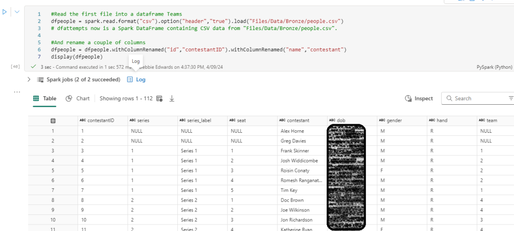
We have used .withColumnRenamed to change a couple of columns.

ID to ContestantID and name to contestant

Before moving on. the assumption is that People is a distinct list.

Lets count the rows in each table so far

row_countp = dfpeople.count()
row_countc = dfcont.count()
print(f"Number of rows in the dfpeople: {row_countp}")
print(f"Number of rows in the dfcont: {row_countc}")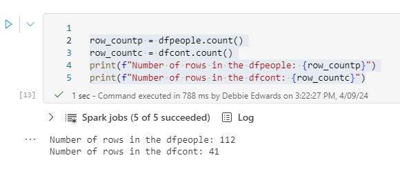

There is a lot more people in our new DataFrame. But are they unique?

#We need to test. Do we have unique Contestants?

#We need to import a function for col
from pyspark.sql.functions import *

dfpeople.groupBy('contestant')\
       .agg(min('contestantID').alias('MinContestantID'),count('contestant').alias('TotalRecords'))\
       .filter(col('TotalRecords')>1).show(1000)

Using \ allows us to break the code onto separate lines

We have the same issue here where some of the people have more than one record so lets filter a few

filtered_df = dfpeople.filter(dfpeople['name'] == 'Liza Tarbuck')
filtered_df.show()

The original assumption in Part 1 was incorrect. We have multiple based on the Champion of Champion series here. So the ID is not for the contestant. it’s for the contestant and series and some people have been on multiple series.

Do the IDs match between the tables?

filtered_df = dfcont.filter(dfcont['contestant'] == 'Bob Mortimer')
filtered_df.show()

Yes. So we need to rethink dim contestants. Actually if they exist in both we only need to use people. So we need to join them and check out if this is the case

Checking values exist in People that we can see in attempts – rename Columns

We want to join the contestants that we obtained the attempts table to dfpeople. Simply so we can check what is missing?

We know we have more in people. But what happens if there are values missing in people than are in attempts? This will cause us more problems.

We will join on the ID and the contestant so before the join. Lets rename the dfCont columns so we don’t end up with duplicate column names

#And rename a couple of columns
dfcont = dfcont.withColumnRenamed("contestantID","cont_contestantID").withColumnRenamed("contestant","cont_contestant")

display(dfcont)

join dfCont and dfPeople

Please note that when joining tables, its better to create a new DataFrame rather than update an original one, because if you have to run it again, the DataFrame you join from will have changed.

# Original condition
original_condition = dfpeople["contestantID"] == dfcont["cont_contestantID"]

# Adding another condition based on the 'name' column
combined_condition = original_condition & (dfpeople["contestant"] == dfcont["cont_contestant"])

# Now perform the left outer join
dfcontcheck = dfpeople.join(dfcont, on=combined_condition, how="full")

display(dfcontcheck)

So we have everything in one table. Lets do some filtering to check our findings

Filter for Null Values

from pyspark.sql import functions as F
dfcontcheck.filter(F.isnull("cont_contestantID")).show(1000)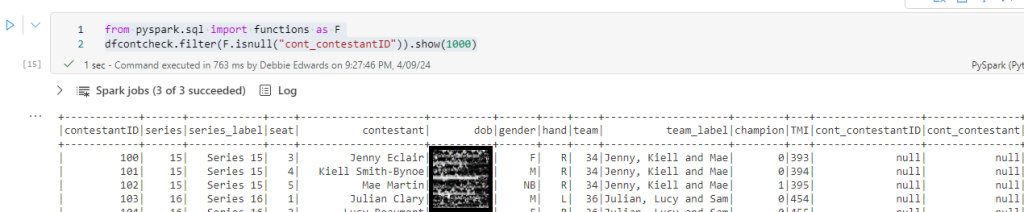

72 records that don’t exist in dfattempt which is fine

from pyspark.sql import functions as F
dfcontcheck.filter(F.isnull("contestantID")).show(1000)

And none in attempts that are in people.

People is therefore our master data set and the PySpark code can be changed accordingly.

At the moment there is a lot of checks happening in the PySpark code. Once up and running and ready to be turned into a proper transformation notebook. All these checks could be removed if required to simplify.

Updating the Code with the new Logic

We are taking the code from Part 1 and completely updating based on the new findings

Start Spark session

%%configure
{
    "defaultLakehouse": {  
        "name": "DebbiesFabricLakehouse"
    }
}

Read People into dfPeople DataFrame

#Read the first file into a dataframe Teams
dfpeople = spark.read.format("csv").option("header","true").load("Files/Data/Bronze/people.csv")
# dfattempts now is a Spark DataFrame containing CSV data from "Files/Data/Bronze/people.csv".

#And rename a couple of columns
dfpeopletransf  = dfpeople.withColumnRenamed("id","contestantID").withColumnRenamed("name","contestant")

print(dfpeopletransf.count())
print(dfpeopletransf.distinct().count())
display(dfpeopletransf.distinct())

.withColumnRenamed brings back the dfpeople data set but renames the specified columns

Create dfCont to create our initial contestants DataFrame

Previously we had a lot of code blocks checking and creating Min IDs for a distinct contestant list. but now we have more of an understanding we can do this with less code.

#Lets immediately do the group by and min value now we know what we are doing to create a distinct list (Removing any IDs for a different series)

#import the function col to use. 
from pyspark.sql.functions import col

#Creates the full distinct list. 

dfcont = dfpeopletransf.groupBy('contestant', 'dob', 'gender','hand' )\
       .agg(min('contestantID').alias('contestantID'),count('contestant').alias('TotalRecords'))


display(dfcont)

groupby. all the distinct values we want. Contestant, dob, gender and hand all are unique with the name. (Previously we just had contestant)

Next we agg (aggregate with min contestantID and cont the number of contestants as total records

If you are used to SQL you would see the following

SELECT MIN(contestantID) AS contestantID, contestant, dob, gender, hand, Count(*) AS TotalRecords
FROM dfpeopletransf
GROUP BY contestant, dob, gender, hand

Create a Current Age

# Create a Spark session
#spark = SparkSession.builder.appName("AgeCalculation").getOrCreate()

# Convert the date of birth column to a date type in dfCont
dfcont = dfcont.withColumn("dob", dfcont["dob"].cast("date"))

# add the current date and set up into a new dataframe
df = dfcont.withColumn("current_date", current_date())

#Calculate age using dob and current date 
df = df.withColumn("age_decimal", datediff(df["current_date"], df["dob"]) / 365)

#Convert from decimal to int  
df = df.withColumn("age", col("age_decimal").cast("int"))

#Convert Customer ID to int
df = df.withColumn("contestantID", col("contestantID").cast("int"))

#Update dfCont
dfcont = df.select("contestantID", "contestant", "dob","gender","hand", "age")

dfcont.show(1000)

It would be fun to filter by Age and Age Group. lets create the age first based on the current Date,

• First of all we ensure date is a date .cast(“date”)
• Then using .withColumn we add the current date to the data frame current_date()
• Next. we use datediff to get the age from the date of birth and the current date
• Set age to int and customerID to int
• Next update dfCont with the full list of columns (Excluding current_date because that was only needed to create the age.

Create Age group

from pyspark.sql import SparkSession
from pyspark.sql.functions import when, col

# Create a Spark session
#spark = SparkSession.builder.appName("ConditionalLogic").getOrCreate()

# Apply conditional logic
dfcont = dfcont.withColumn("ageRange", when(col("age") < 20, "0 to 20")
                               .when((col("age") >= 20) & (col("age") <= 30), "20 to 30")
                               .when((col("age") >= 30) & (col("age") <= 40), "30 to 40")
                               .when((col("age") >= 40) & (col("age") <= 50), "40 to 50")
                               .when((col("age") >= 50) & (col("age") <= 60), "50 to 60")
                               .otherwise("Over 60"))

# Show the result
dfcont.show()

We have created what would be a CASE in SQL

using .WithColumn to create a new column. .when .otherwise are used to create this new data item

Create New Row for -1 NA Default Row

We are back to almost the original code. Creating our Default row but this time with more columns

from pyspark.sql import SparkSession
from pyspark.sql import Row

# Create a sample DataFrame
data = [(-1, "Not Known","1900-01-01","NA","NA","0","NA")]
columns = ["contestantID", "contestant", "dob", "gender", "hand", "age", "ageRange"]
new_row  = spark.createDataFrame(data, columns)

# Union the new row with the existing DataFrame
dfcont = dfcont.union(new_row)

# Show the updated DataFrame
#dfcont.show(1000)

dfcont.show(1000)

We can now see Not known in the list

Running a DISTINCT just in case we applied the above more than once.

#Just in case. We distinct again to remove any extra NA Rows
dfcont = dfcont.distinct()
dfcont.show(1000)

Checking we have unique Contestants GROUPBY

#And lets check the new distinct list with Min IDs we have made
#We need to import a function for col
from pyspark.sql.functions import *

dfcont.groupBy('contestant', 'dob', 'age','ageRange', 'hand','gender')\
        .agg(count('contestant').alias('TotalRecords'))\
        .filter(col('TotalRecords')>1).show(1000)


#Hopefully there should be no records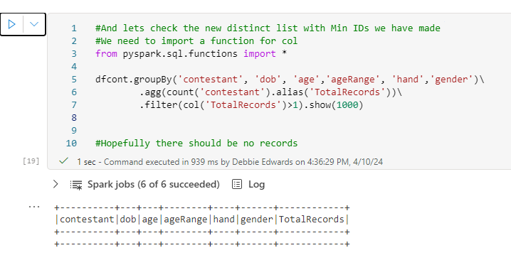

We have all unique contestants, including the extra information we have added to the dimension.

Creating the Contestant Key

We can now create slightly better code than Part 1 using less code blocks

#Now finally for this we need a Key a new column
# Imports Window and row_number
from pyspark.sql import Window
from pyspark.sql.functions import row_number

# Applying partitionBy() and orderBy()
window_spec = Window.partitionBy().orderBy("ContestantID")

# Add a new column "row_number" using row_number() over the specified window
dfcont = dfcont.withColumn("ContestantKey", row_number().over(window_spec)- 2)

# Show the result
dfcont.show(1000)

Previously a partition column with the value 1 was added so we could do the following: .partitionBy(“partition”)

But simply using partitionBy() and not including a column removes the need for the extra code and column and does the same thing.

Adding the Team

Previously the Team was added from attempts.csv but we know that we can change this to people now and have better team information.

#Creates the full distinct list. 
dfContTeam = dfpeopletransf.select(col("contestantID").alias("teamcontestantID"), col("contestant").alias("teamContestant"), 
col("team").alias("teamID"),col("team_label").alias("TeamName")).distinct()

display(dfContTeam)

Remove Rows with Empty team information

#Now remove the rows with null teamids

# Import necessary libraries and create a Spark session
#from pyspark.sql import SparkSession
spark = SparkSession.builder.master("local[1]").appName("SparkByExamples.com").getOrCreate()

# Drop rows with NULL values in the "id" column
dfContTeam = dfContTeam.na.drop(subset=["teamId"])

# Show the filtered DataFrame
dfContTeam.show(truncate=False)

Join team to Contestant

#Now what we want to do is add TeamName into dfcont

dfcont = dfcont.join(dfContTeam, dfcont["contestant"] == dfContTeam["teamContestant"], how="left").drop(dfContTeam.teamContestant).drop(dfContTeam.teamcontestantID)

display(dfcont)

This time we cleaned up the code by adding the two columns to drop in the above statement so we don’t have two names and IDs from both data sets.

Create DELTA PARQUET TABLE

from delta.tables import DeltaTable

dfcont.write.mode("overwrite").format("delta").saveAsTable("dimContestant")

Because we are overwriting our new data set should overwrite our old Dimension. However, there will be conflict issues because the schema is so different so for this exercise, The files will be removed before being re-added.

CREATE PARQUET Table in Files Folder

dfcont.write.mode("overwrite").parquet('Files/Data/Silver/DimContestant.parquet')

We now have options of using the Delta PARQUET, or just the PARQUET File.

Conclusion

In Part 1 we used attempts csv for contestants. For Part 2 we did lots of analysis and checked that actually, people was a better data source for contestants. So we changed the input for the initial DataFrame to people.csv

We also used the opportunity to tidy up the code, now we are getting to grips with Pyspark as an alternative to SQL.

Next on the list is to create more dimensions.

• Dim Task
• Dim Episode
• Dim Date

And the Taskmaster Stats Fact Table

Then to do some analysis, using the inbuilt visuals in a Notebook, and Power BI.